17.1 – Background

In the earlier chapter we had this discussion about the range within which Nifty is likely to trade given that we know its annualized volatility. We arrived at an upper and lower end range for Nifty and even concluded that Nifty is likely to trade within the calculated range.

Fair enough, but how sure are we about this? Is there a possibility that Nifty would trade outside this range? If yes, what is the probability that it will trade outside the range and what is the probability that Nifty will trade within the range? If there is an outside range, then what are its values?

Finding answers to these questions are very important for several reasons. If not for anything it will lay down a very basic foundation to a quantitative approach to markets, which is very different from the regular fundamental and technical analysis thought process.

So let us dig a bit deeper and get our answers.

17.2 – Random Walk

The discussion we are about to have is extremely important and highly relevant to the topic at hand, and of course very interesting as well.

Have a look at the image below –

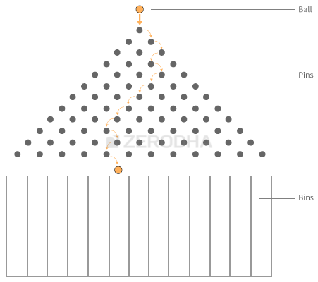
What you see is called a ‘Galton Board’. A Galton Board has pins stuck to a board. Collecting bins are placed right below these pins.

The idea is to drop a small ball from above the pins. Moment you drop the ball, it encounters the first pin after which the ball can either turn left or turn right before it encounters another pin. The same procedure repeats until the ball trickles down and falls into one of the bins below.

Do note, once you drop the ball from top, you cannot do anything to artificially control the path that the ball takes before it finally rests in one of the bins. The path that the ball takes is completely natural and is not predefined or controlled. For this particular reason, the path that the ball takes is called the ‘Random Walk’.

Now, can you imagine what would happen if you were to drop several such balls one after the other? Obviously each ball will take a random walk before it falls into one of the bins. However what do you think about the distribution of these balls in the bins?.

• Will they all fall in the same bin? or
• Will they all get distributed equally across the bins? or
• Will they randomly fall across the various bins?

I’m sure people not familiar with this experiment would be tempted to think that the balls would fall randomly across various bins and does not really follow any particular pattern. But this does not happen, there seems to be an order here.

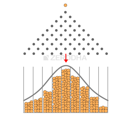
Have a look at the image below –

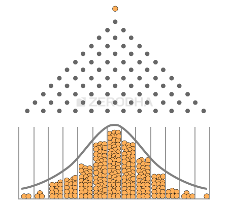
It appears that when you drop several balls on the Galton Board, with each ball taking a random walk, they all get distributed in a particular way –

• Most of the balls tend to fall in the central bin
• As you move further away from the central bin (either to the left or right), there are fewer balls
• The bins at extreme ends have very few balls

A distribution of this sort is called the “Normal Distribution”. You may have heard of the bell curve from your school days, bell curve is nothing but the normal distribution. Now here is the best part, irrespective of how many times you repeat this experiment, the balls always get distributed to form a normal distribution.

This is a very popular experiment called the Galton Board experiment; I would strongly recommend you to watch this beautiful video to understand this discussion better –

So why do you think we are discussing the Galton Board experiment and the Normal Distribution?

Well many things in real life follow this natural order. For example –

• Gather a bunch of adults and measure their weights – segregate the weights across bins (call them the weight bins) like 40kgs to 50kgs, 50kgs to 60kgs, 60kgs to 70kgs etc. Count the number of people across each bin and you end up getting a normal distribution
• Conduct the same experiment with people’s height and you will end up getting a normal distribution
• You will get a Normal Distribution with people’s shoe size
• Weight of fruits, vegetables
• Commute time on a given route
• Lifetime of batteries

This list can go on and on, however I would like to draw your attention to one more interesting variable that follows the normal distribution – the daily returns of a stock!

The daily returns of a stock or an index cannot be predicted – meaning if you were to ask me what will be return on TCS tomorrow I will not be able to tell you, this is more like the random walk that the ball takes. However if I collect the daily returns of the stock for a certain period and see the distribution of these returns – I get to see a normal distribution aka the bell curve!

To drive this point across I have plotted the distribution of the daily returns of the following stocks/indices –

• Nifty (index)
• Bank Nifty ( index)
• TCS (large cap)
• Cipla (large cap)
• Kitex Garments (small cap)
• Astral Poly (small cap)

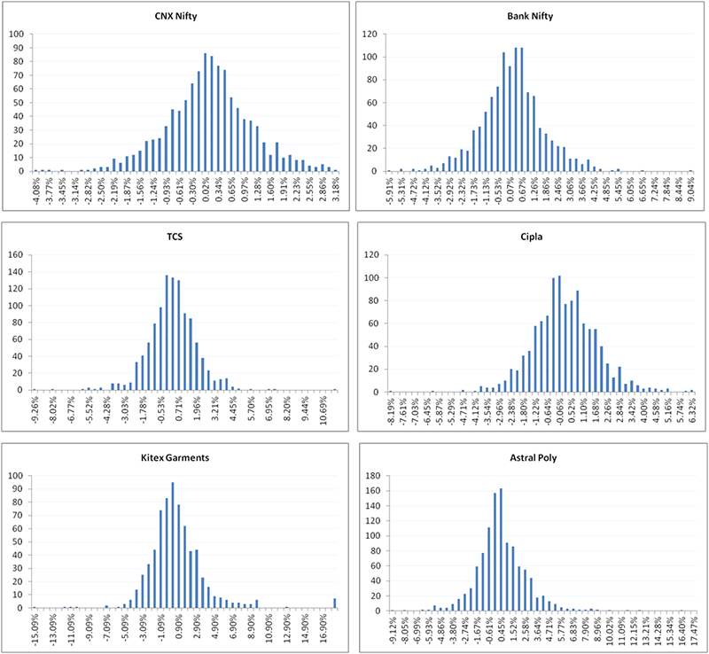
As you can see the daily returns of the stocks and indices clearly follow a normal distribution.

Fair enough, but I guess by now you would be curious to know why is this important and how is it connected to Volatility? Bear with me for a little longer and you will know why I’m talking about this.

17.3 – Normal Distribution

I think the following discussion could be a bit overwhelming for a person exploring the concept of normal distribution for the first time. So here is what I will do – I will explain the concept of normal distribution, relate this concept to the Galton board experiment, and then extrapolate it to the stock markets. I hope this will help you grasp the gist better.

So besides the Normal Distribution there are other distributions across which data can be distributed. Different data sets are distributed in different statistical ways. Some of the other data distribution patterns are – binomial distribution, uniform distribution, poisson distribution, chi square distribution etc. However the normal distribution pattern is probably the most well understood and researched distribution amongst the other distributions.

The normal distribution has a set of characteristics that helps us develop insights into the data set. The normal distribution curve can be fully described by two numbers – the distribution’s mean (average) and standard deviation.

The mean is the central value where maximum values are concentrated. This is the average value of the distribution. For instance, in the Galton board experiment the mean is that bin which has the maximum numbers of balls in it.

So if I were to number the bins (starting from the left) as 1, 2, 3…all the way upto 9 (right most), then the 5^th bin (marked by a red arrow) is the ‘average’ bin. Keeping the average bin as a reference, the data is spread out on either sides of this average reference value. The way the data is spread out (dispersion as it is called) is quantified by the standard deviation (recollect this also happens to be the volatility in the stock market context).

Here is something you need to know – when someone says ‘Standard Deviation (SD)’ by default they are referring to the 1^st SD. Likewise there is 2^nd standard deviation (2SD), 3^rd standard deviation (SD) etc. So when I say SD, I’m referring to just the standard deviation value, 2SD would refer to 2 times the SD value, 3 SD would refer to 3 times the SD value so on and so forth.

For example assume in case of the Galton Board experiment the SD is 1 and average is 5. Then,

• 1 SD would encompass bins between 4^th bin (5 – 1 ) and 6^th bin (5 + 1). This is 1 bin to the left and 1 bin to the right of the average bin
• 2 SD would encompass bins between 3^rd bin (5 – 2*1) and 7^th bin (5 + 2*1)
• 3 SD would encompass bins between 2^nd bin (5 – 3*1) and 8^th bin (5 + 3*1)

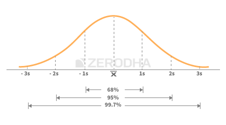
Now keeping the above in perspective, here is the general theory around the normal distribution which you should know –

• Within the 1^st standard deviation one can observe 68% of the data
• Within the 2^nd standard deviation one can observe 95% of the data
• Within the 3^rd standard deviation one can observe 99.7% of the data

The following image should help you visualize the above –

Applying this to the Galton board experiment –

• Within the 1^st standard deviation i.e between 4^th and 6^th bin we can observe that 68% of balls are collected
• Within the 2^nd standard deviation i.e between 3^rd and 7^th bin we can observe that 95% of balls are collected
• Within the 3^rd standard deviation i.e between 2^nd and 8^th bin we can observe that 99.7% of balls are collected

Keeping the above in perspective, let us assume you are about to drop a ball on the Galton board and before doing so we both engage in a conversation –

You – I’m about to drop a ball, can you guess which bin the ball will fall into?

Me – No, I cannot as each ball takes a random walk.  However, I can predict the range of bins in which it may fall

You – Can you predict the range?

Me – Most probably the ball will fall between the 4^th and the 6^th bin

You – Well, how sure are you about this?

Me – I’m 68% confident that it would fall anywhere between the 4^th and the 6^th bin

You – Well, 68% is a bit low on accuracy, can you estimate the range with a greater accuracy?

Me – Sure, I can. The ball is likely to fall between the 3^rd and 7^th bin, and I’m 95% sure about this. If you want an even higher accuracy then I’d say that the ball is likely to fall between the 2^nd and 8^th bin and I’m 99.5% sure about this

You – Nice, does that mean there is no chance for the ball to fall in either the 1^st or 10^th bin?

Me – Well, there is certainly a chance for the ball to fall in one of the bins outside the 3^rd SD bins but the chance is very low

You – How low?

Me – The chance is as low as spotting a ‘Black Swan’ in a river. Probability wise, the chance is less than 0.5%

You – Tell me more about the Black Swan

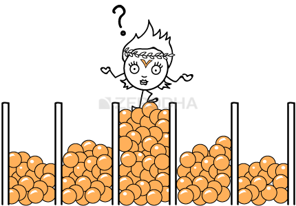
Me – Black Swan ‘events’ as they are called, are events (like the ball falling in 1st  or 10^th bin) that have a low probability of occurrence. But one should be aware that black swan events have a non-zero probability and it can certainly occur – when and how is hard to predict. In the picture below you can see the occurrence of a black swan event –

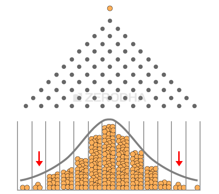
In the above picture there are so many balls that are dropped, but only a handful of them collect at the extreme ends.

17.4 – Normal Distribution and stock returns

Hopefully the above discussion should have given you a quick introduction to the normal distribution. The reason why we are talking about normal distribution is that the daily returns of the stock/indices also form a bell curve or a normal distribution. This implies that if we know the mean and standard deviation of the stock return, then we can develop a greater insight into the behavior of the stock’s returns or its dispersion.     For sake of this discussion, let us take up the case of Nifty and do some analysis.

To begin with, here is the distribution of Nifty’s daily returns is –

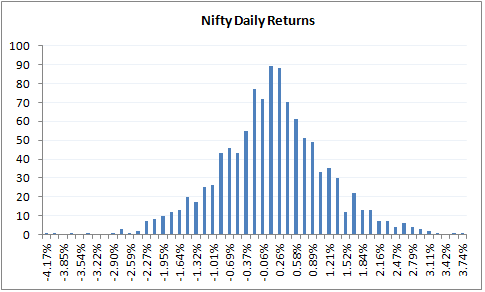
As we can see the daily returns are clearly distributed normally. I’ve calculated the average and standard deviation for this distribution (in case you are wondering how to calculate the same, please do refer to the previous chapter). Remember to calculate these values we need to calculate the log daily returns.

• Daily Average / Mean = 0.04%
• Daily Standard Deviation / Volatility = 1.046%
• Current market price of Nifty = 8337

Do note, an average of 0.04% indicates that the daily returns of nifty are centered at 0.04%. Now keeping this information in perspective let us calculate the following things –

• The range within which Nifty is likely to trade in the next 1 year
• The range within which Nifty is likely to trade over the next 30 days.

For both the above calculations, we will use 1 and 2 standard deviation meaning with 68% and 95% confidence.

Solution 1 – (Nifty’s range for next 1 year)

Average = 0.04%
SD = 1.046%

Let us convert this to annualized numbers –

Average = 0.04*252 = 9.66%
SD = 1.046% * Sqrt (252) = 16.61%

So with 68% confidence I can say that the value of Nifty is likely to be in the range of –

= Average + 1 SD (Upper Range) and Average – 1 SD (Lower Range)
= 9.66% + 16.61% = 26.66%
= 9.66% – 16.61% = -6.95%

Note these % are log percentages (as we have calculated this on log daily returns), so we need to convert these back to regular %, we can do that directly and get the range value (w.r.t to Nifty’s CMP of 8337) –

Upper Range
= 8337 *exponential (26.66%)
= 10841

And for lower range –

= 8337 * exponential (-6.95%)
= 7777

The above calculation suggests that Nifty is likely to trade somewhere between 7777 and 10841. How confident I am about this? – Well as you know I’m 68% confident about this.

Let us increase the confidence level to 95% or the 2^nd standard deviation and check what values we get –

Average + 2 SD (Upper Range) and Average – 2 SD (Lower Range)
= 9.66% + 2* 16.61% = 42.87%
= 9.66% – 2* 16.61% = -23.56%

Hence the range works out to –

Upper Range
= 8337 *exponential (42.87%)
= 12800

And for lower range –

= 8337 * exponential (-23.56%)
= 6587

The above calculation suggests that with 95% confidence Nifty is likely to trade anywhere in the range of 6587 and 12800 over the next one year. Also as you can notice when we want higher accuracy, the range becomes much larger.

I would suggest you do the same exercise for 99.7% confidence or with 3SD and figure out what kind of range numbers you get.

Now, assume you do the range calculation of Nifty at 3SD level and get the lower range value of Nifty as 5000 (I’m just quoting this as a place holder number here), does this mean Nifty cannot go below 5000? Well it certainly can but the chance of going below 5000 is low, and if it really does go below 5000 then it can be termed as a black swan event. You can extend the same argument to the upper end range as well.

Solution 2 – (Nifty’s range for next 30 days)

We know the daily mean and SD –

Average = 0.04%
SD = 1.046%

Since we are interested in calculating the range for next 30 days, we need to convert the same for the desired time period –

Average = 0.04% * 30 = 1.15%
SD = 1.046% * sqrt (30) = 5.73%

So with 68% confidence I can say that, the value of Nifty over the next 30 days is likely to be in the range of –

= Average + 1 SD (Upper Range) and Average – 1 SD (Lower Range)
= 1.15% + 5.73% = 6.88%
= 1.15% – 5.73% = – 4.58%

Note these % are log percentages, so we need to convert them back to regular %, we can do that directly and get the range value (w.r.t to Nifty’s CMP of 8337) –

= 8337 *exponential (6.88%)
= 8930

And for lower range –

= 8337 * exponential (-4.58%)
= 7963

The above calculation suggests that with 68% confidence level I can estimate Nifty to trade somewhere between 8930 and 7963 over the next 30 days.

Let us increase the confidence level to 95% or the 2^nd standard deviation and check what values we get –

Average + 2 SD (Upper Range) and Average – 2 SD (Lower Range)
= 1.15% + 2* 5.73% = 12.61%
= 1.15% – 2* 5.73% = -10.31%

Hence the range works out to –

= 8337 *exponential (12.61%)
= 9457 (Upper Range)

And for lower range –

= 8337 * exponential (-10.31%)
= 7520

I hope the above calculations are clear to you. You can also download the MS excel that I’ve used to make these calculations.

Of course you may have a very valid point at this stage – normal distribution is fine, but how do I get to use the information to trade? I guess as such this chapter is quite long enough to accommodate more concepts. Hence we will move the application part to the next chapter. In the next chapter we will explore the applications of standard deviation (volatility) and its relevance to trading. We will discuss two important topics in the next chapter (1) How to select strikes that can be sold/written using normal distribution and (2) How to set up stoploss using volatility.

Of course, do remember eventually the idea is to discuss Vega and its effect on options premium.

---

Key takeaways from this chapter

1. The daily returns of the stock is a random walk, highly difficult to predict
2. The returns of the stock is normally distributed or rather close to normal distribution
3. In a normal distribution the data is centered around the mean and the dispersion is measured by the standard deviation
4. Within 1 SD we can observe 68% of the data
5. Within 2 SD we can observe 95% of the data
6. Within 3 SD we can observe 99.5% of the data
7. Events occurring outside the 3^rd standard deviation are referred to as Black Swan events
8. Using the SD values we can calculate the upper and lower value of stocks/indices