
15.1 – Background
Having understood Delta, Gamma, and Theta, we are now at all set to explore one of the most interesting Option Greeks – The Vega. Vega, as most of you might have guessed is the rate of change of option premium concerning the change in volatility. But the question is – What is volatility? I have asked this question to quite a few traders, and the most common answer is “Volatility is the up-down movement of the stock market”. If you have a similar opinion on volatility, then it is about time we fixed that ☺.
So here is the agenda, I suppose this topic will spill over a few chapters –
- We will understand what volatility really means
- Understand how to measure volatility
- Practical Application of volatility
- Understand different types of volatility
- Understand Vega
So let’s get started.
15.2 – Moneyball
Have you watched this Hollywood movie called ‘Moneyball’? It’s a real-life story, Billy Beane – manager of a baseball team in the US. The movie is about Billy Beane and his young colleague, and how they leverage the power of statistics to identify relatively low profile but extremely talented baseball players. A method that was unheard of during his time, and a method that proved to be both innovative and disruptive.
You can watch the trailer of Moneyball here.
I love this movie, not just for Brad Pitt, but for the message it drives across on topics related to life and business. I will not get into the details now, however, let me draw some inspiration from the Moneyball method, to help explain volatility :).
The discussion below may appear unrelated to stock markets, but please don’t get discouraged. I can assure you that it is relevant and helps you relate better to the term ‘Volatility’.
Consider 2 batsmen and the number of runs they have scored over 6 consecutive matches –
| Match | Billy | Mike |
|---|---|---|
| 1 | 20 | 45 |
| 2 | 23 | 13 |
| 3 | 21 | 18 |
| 4 | 24 | 12 |
| 5 | 19 | 26 |
| 6 | 23 | 19 |
You are the captain of the team, and you need to choose either Billy or Mike for the 7th match. The batsman should be dependable – in the sense that the batsman you choose should be in a position to score at least 20 runs. Whom would you choose? From my experience, I have noticed that people approach this problem in one of the two ways –
- Calculate the total score (also called ‘Sigma’) of both the batsman – pick the batsman with the highest score for the next game. Or…
- Calculate the average (also called ‘Mean’) number of scores per game – pick the batsman with a better average.
Let us calculate the same and see what numbers we get –
- Billy’s Sigma = 20 + 23 + 21 + 24 + 19 + 23 = 130
- Mike’s Sigma = 45 + 13 + 18 + 12 + 26 + 19 = 133
So based on the sigma, you are likely to select Mike. Let us calculate the mean or average for both the players and figure out who stands better –
- Billy = 130/6 = 21.67
- Mike = 133/6 = 22.16
So it seems from both the mean and sigma perspective, Mike deserves to be selected. But let us not conclude that yet. Remember the idea is to select a player who can score at least 20 runs, and with the information that we have now (mean and sigma), there is no way we can conclude who can score at least 20 runs. Therefore, let’s do some further investigation.
To begin with, for each match played, we will calculate the deviation from the mean. For example, we know Billy’s mean is 21.67, and in his first match, Billy scored 20 runs. Therefore deviation from mean from the 1st match is 20 – 21.67 = – 1.67. In other words, he scored 1.67 runs lesser than his average score. For the 2nd match, it was 23 – 21.67 = +1.33, meaning he scored 1.33 runs more than his average score.
Here is the diagram representing the same (for Billy) –
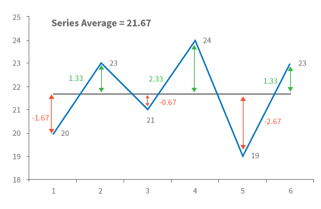
The middle black line represents the average score of Billy, and the double arrowed vertical line represents the deviation from the mean, for each of the match played. We will now go ahead and calculate another variable called ‘Variance’.
Variance is simply the ‘sum of the squares of the deviation divided by the total number of observations’. This may sound scary, but it’s not. We know the total number of observations, in this case, happens to be equivalent to the total number of matches played, hence 6.
So variance can be calculated as –
Variance = [(-1.67) ^2 + (1.33) ^2 + (-0.67) ^2 + (+2.33) ^2 + (-2.67) ^2 + (1.33) ^2] / 6
= 19.33 / 6
= 3.22
Further, we will define another variable called ‘Standard Deviation’ (SD) which is calculated as –
std deviation = √ variance
So the standard deviation for Billy is –
= SQRT (3.22)
= 1.79
Likewise, Mike’s standard deviation works out to be 11.18.
Let’s stack up all the numbers (or statistics) here –
| Statistics | Billy | Mike |
|---|---|---|
| Sigma | 130 | 133 |
| Mean | 21.6 | 22.16 |
| SD | 1.79 | 11.18 |
We know what ‘Mean’, and ‘Sigma’ signifies, but what about the SD? Standard Deviation generalizes and represents the deviation from the average.
Here is the textbook definition of SD “In statistics, the standard deviation (SD, also represented by the Greek letter sigma, σ) is a measure that is used to quantify the amount of variation or dispersion of a set of data values”.
Please don’t get confused between the two sigma’s – the total is also called sigma represented by the Greek symbol ∑ and standard deviation is also sometimes referred to as sigma represented by the Greek symbol σ.
One way to use SD is to project how many runs Billy and Mike are likely to score in the next match. To get this projected score, you need to add and subtract the SD from their average.
| Player | Lower Estimate | Upper Estimate |
|---|---|---|
| Billy | 21.6 – 1.79 = 19.81 | 21.6 + 1.79 = 23.39 |
| Mike | 22.16 – 11.18 = 10.98 | 22.16 + 11.18 = 33.34 |

These numbers suggest that in the upcoming 7th match Billy is likely to get a score anywhere in between 19.81 and 23.39 while Mike stands to score anywhere between 10.98 and 33.34. Because Mike has a wide range, it isn’t easy to figure out if he is going to score at least 20 runs. He can either score 10 or 34 or anything in between.
However, Billy seems to be more consistent. His range is smaller, which means he will neither be a big hitter nor a lousy player. He is expected to be consistent and is likely to score anywhere between 19 and 23. In other words – selecting Mike over Billy for the 7th match can be risky.
Going back to our original question, which player do you think is more likely to score at least 20 runs? By now, the answer must be clear; it has to be Billy. Billy is consistent and less risky compared to Mike.
So in principle, we assessed the riskiness of these players by using “Standard Deviation”. Hence ‘Standard Deviation’ must represent ‘Risk’. In the stock market world, we define ‘Volatility’ as the riskiness of the stock or an index. Volatility is a % number as measured by the standard deviation.
I’ve picked the definition of Volatility from Investopedia for you – “A statistical measure of the dispersion of returns for a given security or market index. Volatility can either be measured by using the standard deviation or variance between returns from that same security or market index. Commonly higher the standard deviation, higher is the risk”.
Going by the above definition, if Infosys and TCS have the volatility of 25% and 45% respectively, then clearly Infosys has less risky price movements when compared to TCS.
15.3 – Some food for thought
Before I wrap this chapter, let’s make some prediction –
Today’s Date = 15th July 2015
Nifty Spot = 8547
Nifty Volatility = 16.5%
TCS Spot = 2585
TCS Volatility = 27%
Given this information, can you predict the likely range within which Nifty and TCS will trade 1 year from now?
Of course we can, let us put the numbers to good use –
| Asset | Lower Estimate | Upper Estimate |
|---|---|---|
| Nifty | 8547 – (16.5% * 8547) = 7136 | 8547 + (16.5% * 8547) = 9957 |
| TCS | 2585 – (27% * 2585) = 1887 | 2585 + (27% * 2585) = 3282 |
So the above calculations suggest that in the next 1 year, given Nifty’s volatility, Nifty is likely to trade anywhere between 7136 and 9957 with all values in between having the varying probability of occurrence. This means to say on 15th July 2016 the probability of Nifty to be around 7500 could be 25%, while 8600 could be around 40%.
This leads us to an exciting platform –
- We estimated the range for Nifty for 1 year; similarly, can we estimate the range Nifty is likely to trade over the next few days or the range within which Nifty is likely to trade upto the series expiry?
- If we can do this, then we will be in a better position to identify options that are likely to expire worthless, meaning we could sell them today and pocket the premiums.
- We figured the range in which Nifty is likely to trade in the next 1 year as 7136 and 9957 – but how sure are we? Is there any degree of confidence while expressing this range?
- How do we calculate Volatility? I know we discussed the same earlier in the chapter, but is there an easier way? Hint – we could use MS Excel!
- We calculated Nifty’s range estimating its volatility as 16.5%, what if the volatility changes?
Over the next few chapters, we will answer all these questions and more!
Key takeaways from this chapter
- Vega measures the rate of change of premium concerning the change in volatility.
- Volatility is not just the up-down movement of markets.
- Volatility is a measure of risk.
- Volatility is estimated by the standard deviation.
- Standard Deviation is the square root of the variance.
- We can estimate the range of the stock price, given its volatility.
- Larger the range of stock, higher is its volatility aka risk.
Its based on a statistical function called ’Cumulative Distribution Function’ abbreviated as CDF. you will touch upon this topic soon.
Hi, I wanted to know the daily volatality & Annual volatality for nifty , how do I find the same or where can i get those numbers?
I guess you can check Sensibull for this. Or NSE itself publishes this data, please do check their daily files.
Standard deviation (SD) is in the form of percentage . ABC stock\’s SD is 10 and stock is trading at 100 meaning lower estimate is 90 and upper estimate is 110 . My question is for Billy\’s case upper estimation, Loss = Investment * (1-SD) 21.6*(1-1.79%) = 21.21 and upper estimation 21.6*(1+1.79%) = 21.99. but why it is 21.6 – 1.79 = 19.81 and 21.6 + 1.79 = 23.39
Typing correction *
Standard deviation (SD) is in the form of percentage . ABC stock’s SD is 10 and stock is trading at 100 meaning lower estimate is 90 and upper estimate is 110 . My question is for Billy’s case lower estimation Investment*(1-SD) 21.6*(1-1.79%) = 21.21 and upper estimation Investment*(1+SD) 21.6*(1+1.79%) = 21.99. but why it is 21.6 – 1.79 = 19.81 and 21.6 + 1.79 = 23.39
The confusion stems from mixing up absolute numbers with percentages.
In Billy’s case, when we calculated the standard deviation, we got 1.79 runs. This is an absolute number, not a percentage. Billy scores runs, right? So his SD is also in runs. When you want to estimate his range for the next match, you simply add and subtract this SD from his average:
Lower estimate = 21.6 – 1.79 = 19.81 runs
Upper estimate = 21.6 + 1.79 = 23.39 runs
Now, when it comes to stocks, we express volatility as a percentage. If ABC stock’s SD is 10%, it means the stock’s price can move up or down by 10% from its current level. So naturally, the calculation becomes:
Lower estimate = 100 × (1 – 0.10) = 90
Upper estimate = 100 × (1 + 0.10) = 110
The formula you’re mentioning – Investment × (1 ± SD%) – is absolutely correct when SD is expressed as a percentage. But in Billy’s case, the 1.79 is not a percentage; it’s an absolute value in runs.
Think of it this way: if Billy scores runs, his SD is in runs. If a stock moves in price, its SD is expressed as a percentage of that price.
Now, if you really wanted to convert Billy’s SD into a percentage (though it’s not necessary for the example), you’d do: (1.79 ÷ 21.6) × 100 = 8.29%. Then if you calculate using your formula:
21.6 × (1 – 0.0829) = 19.81
21.6 × (1 + 0.0829) = 23.39
Same answer, different route!
The key takeaway here is this: when your SD is an absolute number, add/subtract directly. When it’s a percentage, multiply using the (1 ± SD%) formula.
Hope this clears things up! And remember, once you get your head around this concept, everything else in options and volatility becomes much easier to digest.
Good luck!
Given this information, can you predict the likely range within which Nifty and TCS will trade 1 year from now?
Of course we can, let us put the numbers to good use –
Asset Lower Estimate Upper Estimate
Nifty 8547 – (16.5% * 8547) = 7136 8547 + (16.5% * 8547) = 9957
TCS 2585 – (27% * 2585) = 1887 2585 + (27% * 2585) = 3282
So the above calculations suggest that in the next 1 year, given Nifty’s volatility, Nifty is likely to trade anywhere between 7136 and 9957 with all values in between having the varying probability of occurrence. This means to say on 15th July 2016 the probability of Nifty to be around 7500 could be 25%, while 8600 could be around 40%.
Sir I couldn’t find any explanation related to my question as you say.Will you please be kind enough to explain/ elaborate?
Hiren, the whole of this chapter is geared towards explaining this 🙂
But anyway, please do share your question again, I can check.
How one could arrive at conclusion that on 15 th July 2016 the probability of Nifty be around 7500 could be 25% while 8600 could be around 40%?
Hmm, based on the properties of normal distribution. We have discussed this in the chapter and the subsequent comments. Please do check.
Hi Karthik,
\”So the above calculations suggest that in the next 1 year, given Nifty’s volatility, Nifty is likely to trade anywhere between 7136 and 9957 with all values in between having the varying probability of occurrence. This means to say on 15th July 2016 the probability of Nifty to be around 7500 could be 25%, while 8600 could be around 40%.\”
How you calculated this 25% and 40% values in the above pharagraph?
Regards,
Pavit Kapoor
This is based on the property of normal distribution.
First of all, thanks for this great series.
I have a question, generally we divide sum of the squares of the deviation by (n-1) where n is number of observations, to calculate variance. why did you divide by total number of observations here.
Thats the formula, I\’m sure there is a derivation for that. I\’m not aware of it though.
How you calculate the probability of nifty to be around 7500 is 25% and 8600 is 40% ?
Hey, I\’ve explained this in the chapter Niraj. Please do check. Will be happy to explain post that 🙂
sir can you explain why you multiply with exponential to the market price instaed of doing market price (1 +or- %)
That is to convert log to regular scale.
sir in some examples you calculate range with in directly without using daily mean .. then how to the percentage of confidence weather 68% or 95% or 99%
Using the properties of normal distribution.
This means to say on 15th July 2016 the probability of Nifty to be around 7500 could be 25%, while 8600 could be around 40% , how you got into this 25% & 40% probability sir
I\’ve explained this in the chapter. Basically based on the normal distribution properties.
Dear Sir,
Please share the excel, it is not downloadable.
Thanks,
Ashish
Can you try downloading from another browser?
\”This means to say on 15th July 2016 the probability of Nifty to be around 7500 could be 25%, while 8600 could be around 40%.\” – i could not understand this sentence please elaborate.
Hey Shubham, these are odds that we calculate based on normal distribution property. Have explained in the chapter itself.
Hi
My question is, taking all that you have taught us on greeks, how could we use it to calculate an appropriate entry point to buy a call/put, ie. apart from using oi, coi, volume data
I really enjoy reading your material
Thanks Rohit. I\’ve explained the application of greeks separately. Do check that 🙂
Karthikjii
How you done the series average chart.i want do in excel for keep im my mind forever 😉
Not sure if I understand your query fully, Abdulla. Can you please elaborate? Thanks.
How did you made the calculation based on the data that you said
\”on 15th July 2016 the probability of Nifty to be around 7500 could be 25%, while 8600 could be around 40%.\”
This is much confusing.
Siva, we have explained this in detail in the chapter itself. Request you to check that followed by the comments.
Hi Sir – How did you calculate the probabilities here to be 35% and 40% when NIFTY is around 7500 & 8600 ?
\”So the above calculations suggest that in the next 1 year, given Nifty’s volatility, Nifty is likely to trade anywhere between 7136 and 9957 with all values in between having the varying probability of occurrence. This means to say on 15th July 2016 the probability of Nifty to be around 7500 could be 25%, while 8600 could be around 40%.\”
This is written towards end of volatility calculation of NIFTY and TCS example.!
Naveen, this is by keeping the probability of normal distribution in perspective. I\’ve explained this in the chapter itself.
In the above example \”This means to say on 15th July 2016 the probability of Nifty to be around 7500 could be 25%, while 8600 could be around 40%.\”
It would be very much helpful if you can explain how the probability is calculated?
Its based on the normal distribution of stock prices, Ansha. I\’ve explained this in the chapter itself.
* I have gone through the comment section , I tried to do this in excel with (norm.dist) function
the nifty spot is 8547
the volatility is 16.5%
SD = NIFTY SPOT*VOLATILITY =1410.25
I applied norm.dist function =norm.dist(price to check \”7500\”,nifty spot\”8547\”,sd\”1410.25\”,true)
= 22.89%
Is this the way to find the percentage ?🙂
YOu can easily do this on Excel, no need for manual calculation 🙂
\”Nifty is likely to trade anywhere between 7136 and 9957 with all values in between having the varying probability of occurrence. This means to say on 15th July 2016 the probability of Nifty to be around 7500 could be 25%, while 8600 could be around 40%.\” Hi sir, Here I could not get the formula derivation of (\”getting 25% and 40% values\”).
please help me🙂
Swarnava, this is based on the normal distribution property of the returns of the stock/index. Please do check the chapter, I\’ve tried to explain this 🙂
Sir, how did you know in the above example that the probability of Nifty to be around 7500 could be 25%, while 8600 could be around 40% (15.3 for your reference). Please explain!
Thats the chapter about, Deepak 🙂
good
Hello, first of all, thanks for the great content.
One quick question- I\’ve noticed that sometimes, the index chart goes up while ITM(CE) option goes down and vice versa i.e. index goes down but option ITM(CE) goes up. could you explain what is the underline reason for that ?
Thanks
Maybe this was close to the expiry date?
Thank you! 🙂
Happy learning!
Especially putting this Comment section has been very useful for me, after going through the whole chapter almost all the querries rose in mind can be resolved by going through this QnA session.
Regards
Thats the idea of having comments, happy learning 🙂
Hi Karthik,
Good Day,
I understood that volatility represents risk, but I am unable to understand what is the risk relating to? Risk of what? Risk of stock falling in price? or something else.
Also, I understood higher volatility means, bigger price range in which stock or index can trade for the given period of time. Im such cases, higher volatility is better isn\’t it? because when the range is bigger, it gives better opportunities to trade in a day.
Can you please help me out in this regard.
Thank You.
Risk is the stock\’s price moving away from its average expected price. The higher the divergence, the higher the risk.
Thanks for answering. Yes Sir, I can understand that. You mentioned that in certain instances that market has bounced back when VIX was lower. But isn\’t that the usual scenario considering the negative correlation between VIX and NIFTY. So that is why I\’m asking in that case if VIX increases, the market usually goes down. Am I right? Because whenever I read about high volatility, I always assumed that high volatility can happen in both uptrend and downtrend. But this negative correlation says otherwise. Kindly clarify my doubt sir.
Thats right. The usual behavior is that with increasing ViX, the markets tend to go down as the fear component increases in the market.
I mean I\’m asking the above question from the aspect of a single option buyer without any strategies. Then in that case, he will benefit only from put options when VIX increases right? Because we want volatility to increase for option buyers to gain and by that logic if volatility increases, then market will have to fall and only in that scenario will an option buyer gain. Please correct me if my assumptions are wrong.
Ah ok. I thought you were asking from a generic market perspective. Option premiums (both call and put) increase when volatility increases. An increase in volatility benefits the buyer, and a decrease in volatility helps the seller.
Sir, If VIX INDEX increases, does that only mean that market has high chance to go down? Or can markets go higher in high volatile situations also? I understand the correlation between NIFTY and VIX. But in case if there are only higher chances that market goes down if VIX increases, does that mean we should only look for shorting opportunities at that time?
No, VIX is a measure of volatility. But it need not always mean that the market will go down. There have been situations where ViX has stayed low but markets have bounced.
Please indicate the volatility ranges for CE & PE for intraday trading of Nifty50 & Banknifty.
Please do check the volatility cone, you will get a perspective of the range.
Please indicate the volatility ranges for CE & PE.
There is no indicative range that will fit all options.
For Eg. It stock is in negative trend. And if we take 1 year of closing price and calculate average. It will be in negative.
So naturally Annual Average will go negative. So how to calculate
Average + 1 SD (Upper Range) and Average – 1 SD (Lower Range)
Agree, in such cases, traders usually tend to take short timeframes.
Sorry, my bad, I think chapter talks about Summation notation that is also known as Sigma operator.
Yeah, sigma as in \’sum of all\’, is the context used in this chapter.
Term \”Sigma\” is used to denote standard deviation SD, and not absolute total score as mentioned in the chapter. Sigma signifies the consistency, so captain will select person with less SD or Sigma.
Hello,sir can you help me with this;
This means to say on 15th July 2016 the probability of Nifty to be around 7500 could be 25%, while 8600 could be around 40%.
How is this calculated ?
Ah, this is based on the range calculation using the normal distribution method.
Hi Kartik ,
Great explanation was wondering how did we come up with the probability of the NIFTY values did we assume that or is there any relation to Volatility?
Its basis the assumption that the returns are normally distributed and hence follow the principle of standard deviation.
Dear Karrhik sir,
I couldn\’t get when you said \”its context-based\”. Could you please explain a bit ?
When you say other volatilities you mean Historical Volatility, Forecasted Volatility, Implied Volatility (IV) ?
Again, its context-based 🙂
Dear Karthik sir
What is the role of annualized volatility? Where is it used? Calculating volatility for 1 month or a week is understood.
We can\’t hold the option uptil 1 year. So kindly explain. Thanks.
All other volatilities are derived from the annualized volatility, Sandeep. So even if you don\’t hold for 1 year, you need that to calculate shorter volatilities.
How you come across the conclusion that change is for 1 year. In the calculation there is nothing related to time
The look back period is 1 year right?
\”This means to say on 15th July 2016 the probability of Nifty to be around 7500 could be 25%, while 8600 could be around 40%\”- How sir?
We discussed the standard deviation and probability distribution (normal distribution) right? Its basis that.
Dear Karthik sir,
The volatility that we have discussed in this chapter is the Implied Volatility or Implied Volatility is something different ?
Thanks
We are discussing historical volatility here, will move to implied volatility in the next chapter I guess.
Thanks sir. So if the 1SD = 16.5% then can we say that 2SD will be 33% and 3SD will be 49.5% right sir?
Yes, thats right.
Dear Karthik sir,
You have said in the chapter that volatility is a % number as measured by the Standard Deviation.
Now suppose Nifty volatility is 16.5% what would be the Standard Deviation ?
Thanks
16.5% is the 1SD of Nifty, which as you know is the volatility.
Dear Karthik sir,
Could you please add the above said Cumulative Distribution Function (CDF ) to the chapter?
or add it to the end of this module. Thanks a lot.
Will try and do that Sandeep.
Dear Karthik sir,
In one of the above comments you talked of Cumulative Distribution Function.
\”Its based on a statistical function called ‘Cumulative Distribution Function‘ abbreviated as CDF. I will touch upon this topic soon.\”
In which chapter have you talked about this concept? Please let me know.
Thanks
Ah, I may have skipped it Sandeep.
Thank You Karthik ji for reply. Eagerly waiting for solution/guidance on my both the queries.
Will do.
Thank you Karthik Ji and team.
I would like to call you ‘PANDIT ’, coz pserson who is able to give us a deep insight into a subject is called Pandit
I am new to stock market world, whatever I know about stock market world, it’s because of you & Zerodha Varsity team. Thank you so much.
I have been reading modules available on this platform. I have few doubts in Option Theory, instead of annoying you about repeated question, I spent almost 10-12 hours reading all the 1914 comments, I found only 3-4 traders raised doubt regarding my Query No.1 (as follows) and you responded that you will look into this and reply. But I think still this query is unanswered. So I decided to put into the comments. I know you might be busy, but I request you to please find some time and solve this query.
Query 1:
a) In section 15.3 you have calculated Nifty & TCS lower range and upper range by directly subtracting and adding S.D. from their respective spot prices respectively (without adding/subtracting volatility to average value and doing rest of the calculations) {Eg. from section 15.3 is as: 8547-(16.5%*8547)=7136 & 8547+(16.5%*8547)=9957}
b) In section 17.4, you have calculated Nifty’s range for next 1 year with 68% & 95% confidence. Here you have added and subtracted 1SD or 2SD to Nifty’s average value and then you have taken exponential of these two (as we have calculated S.D. with Log to the base ‘e’) and multiplied to the spot price to get Nifty’s range for next 1 year. {Eg. from section 17.4 is as: 8337*exp (1.15%+5.73%)= 8930 & 8337*exp(1.15%-5.73%)=7963}
c) In section 18.1, you have calculated Nifty’s range till expiry (for 16 days) with 68% confidence. Here you have added and subtracted 1SD to Nifty’s average value and then without taking exponential of these two %, you have directly added & subtracted these % to Nifty’s spot price. {Eg. from section 18.1 is as: 8462 [1+(0.65%+3.567%)]=8818 & 8462 [1+(0.65%-3.567%)]= 8214}
Here are some observations:
Point 1: In a) & b) you have directly added/subtracted % to spot price to get the range, but there is slight difference between these two. In a) you haven’t added/subtracted S.D. to average value & calculated range and In b) you have added/subtracted S.D. to average value & calculated range. {e.g. from Section 17.4 : 1.15% +5.73%= 6.88% & 1.15%-5.73%=-4.58%}
Point 2: In b) & c) you have added/subtracted S.D. to average to calculate range, but difference between these two is as: In b) you have taken exponential of % and calculated the range of Nifty {e.g. from Sect 17.4 : 8337*exp (1.15%+5.73%)= 8930 } in c) you haven’t taken exponential of % to calculate range of Nifty. (eg. from section 18.1 : 8462 [1+(0.65%+3.567%)]=8818}
Point 3: average % is not taken with function of ‘Log’ to the base ‘e’, while calculating S.D. %, it is taken with function of ‘Log’ to the base ‘e’ (section 16.1). So how can we add these two % (average & S.D.) directly?
So kindly clarify which method to use.
Whether we should add/subtract S.D. to average OR not???? And accordingly which calculation method to use, with spot price multiplied by Exponential of % OR spot price should directly be multiplied by % to get range. (spot price shouldn\’t be multiplied by exponential of %)
Query 2:
In section 18.2, you expect airtel trade to materialize over next 5 trading session. I have heard this from many persons that they expect particular stock XYZ to hit the target with certain ‘T’ (suppose) time period/trading sessions. So I want to know how one can predict or expect particular stock to materialize with certain trading sessions.??? Your guidance on this please.
Please please please solve query no. 1 & your guidance on query no. 2 (as usual). Thank you in advance.
Nagesh, I\’ve noted your query. I understand the confusion. Please allow me to think through the best possible explanation. Will try and post my reply to this soon.
Here are the exact steps to calculate the price range –
1) Calculate the daily log returns
2) Calculate the mean and SD
3) 68% confidence interval is – Current Price * Exp (mean*time +/- SD *Sqrt (time))
4) 95% confidence interval is – Current Price * Exp (mean*time +/- 2*SD *Sqrt (time))
The process in computationally intensive as it involves the calculation of mean, log returns, exponential etc. You can approximate it with simpler calculations –
1) For short time period (say for 1 year data), the (Mean*time) is so small that it hardly makes any difference to the final value i.e. Mean * time << SD * Sqrt (time)
2) When daily % movements 20%, then calculate using the accurate method.
Will you please describe the process of probability calculation of 25% and 40% mentioned in the chapter.
The probability is because the returns are normally distributed and therefore the laws of normal distribution apply.
Thanks for the clarification Karthik sir.
Good luck!
Hello Sir!
As we have discussed till now the option buyer and seller both play with premiums to earn profits.
However my question was if I am a seller of deep OTM option with a premium of Rs.5 I am entitled to receive Rs.5,however to square off the position I would be buying it again.If the premium remains the same Rs.5 does that mean I am in no profit no loss position?
Example:-
1)Premium:-Rs.5
On the day of expiry:-Rs.5
No profit no loss
2)On the day of expiry:-Rs.3
Short at 5
Purchased back at 3
Rs.5-3=Rs.2 per share profit.
Please guide for the same
Thanks in Advance!
Yes, that\’s correct Paras. So the maximum profit you make here is Rs.5.
No, my question is that in the Billy and Mike cricket score example, why do we have to calculate the projected score as
Avg score +- SD instead of doing Current match score +- SD ?
In Billy and Mike\’s case, the data points were less. Taking Avg + SD makes sense. Does not make intuitive sense in doing avg+SD for markets where the look back period can stretch to 1 year or more.
Dear Karthik sir
In the Billy and Mike cricket score example, why do we have to calculate the projected score as
Avg score +- SD whereas we could also calculate as Current match score +- SD just the same
way in case of Nifty example we are using current Spot price +- SD?
Yes, that\’s right. We take the current spot rate and add & subtract the SDs.
1. Which according to you gives more accurate prediction?
Avg spot price +- SD or Current spot price +- SD?
2. The volatility that you have used is 16.5%. I believe it is annual volatility.
My doubt is that for the calculation of 1 year volatility, 1 year Nifty prices
(historical) need to be taken into consideration right?
1) How will you take average spot? Current spot is good 🙂
2) Yes, that\’s right. Yes, at least 1 year data is needed.
You predicted the Nifty price 1 year from now.
For that you added and subtracted from the current price 8547 [8547 +- SD] (SD = Standard deviation).
But in case of Mike and Billy example, you have used [Avg runs +- SD]
So my question is, in case of Nifty price, we should do Avg price +- SD ?
Its slightly different, you need to consider the current price of Nifty.
Dear Karthik sir,
Referring to section 15.3 example.
Nifty Spot = 8547
Volatility = 16.5%
You have calculated the Upper limit as 8547 + (16.5% * 8547) = 9957
and lower limit as 8547 – (16.5% * 8547) = 7136
Here are some of my questions :
1. To calculate the Upper/Lower limit the Average has to be added or subtracted from.
In the above calculation, 8547 is not the average price, right? So the calculation is wrong?
2. You have predicted the price for the next year. In such case, the average needs to calculated first.
So for that the prices for 1 year have to be taken into consideration?
Please clarify.
1) From the current spot market rate
2) Not sure if I understood the query. But from what I understand, its not really required, why would you need that?
I want to know about an Indicator provided in the Chart namely Standard Deviation Indicator. I want to know about the indicator as I am not able to find satisfactory information about the Standard Deviation Indicator.
Kindly provide comprehensive details about standard Deviation. What can we interpret when SD is 1 or 10 or 40 or 80 or 150. What can we infer with respect to the price of stock if SD is :
1. High for short term
2. High for a long time
3. Low for long term
4. Low for a short time
What can we expect when we combine RSI with SD? What SD tells with respect to volatility and price? Is there any range for SD ?
Also what is the best input or settings for SD? Like what should be period with respect to deviations or if deviation is 2 then what should be period?
Sometimes the SD indicator is 90, sometimes it is less than 10. How can we interpret this indicator?
How can we determine Volatility of an Stock using Standard Deviation Indicator?
on 15th July 2016 the probability of Nifty to be around 7500 could be 25%, while 8600 could be around 40%., how????? calculation plz
Radhe, please do check the explanation in the chapter.
Karthik I got that the possibility of nifty trading at 8600 is a little over 40% and it is derived from cumulative distribution function. But why we take cumulative distribution function instead of probability distribution function? Our probability distribution function is our normal distribution curve and if we take the value pf 8600 in probability distribution function, the value is completely different from the value we get following Cumulative distribution function. Can you please help here?
Nice Analogy, easy to grasp and remember
Happy learning!
Not only this chapter but whole varsity is written in such a manner that there\’s no way one can\’t understand it! Hats off to you Karthik sir!
Here is my question:
I am completely new to option trading so what should be my ideal steps to be more professional, more accurate and obviously more profitable with time in options? Apart from technical perspective, what things should I follow and what should be the path forward?
Thank you!
Thanks for the kind words, Dhananjay.
From what I\’ve noticed, good options traders often combine elements of both TA and FA. Besides, they understand the nuances of options very well. More often they deal with option writing using spreads compared to naked option buying. With time, you will get this too 🙂
Thank you Karthik for quick reply. I have gone through that chapter. Yes we can say like there is 68% likelihood of NIFTY trading between 7136 and 9957 after one year. But in that chapter you didn\’t mention anything how to derive the probability of occurrence of any data within the range. I have seen the graph of cdf of a bell curve. It is hard to understand that 7500 is actually 25% from the graph. If you dig it down a bit further on this it will be very helpful for me and for others as well.
Rahul, these percentage figures are from our regular interpretation of normal distribution. I\’d suggest you look at some study material on normal distribution properties and get a sense of how these are calculated. Once you do, you will understand the basis of these percentages.
Under \”food for thought\” you mentioned that \”Nifty is likely to trade anywhere between 7136 and 9957 with all values in between having the varying probability of occurrence.\” And then you said the chance of nifty trading at 7500 is 25% and at 8600 is 40%. Can you please show how you derived it? The calculation.
Rahul, the calculation is on the basis of normal distribution. Have explained that as well.
great imformation .thanks . CAN i translate in Marathi
Couldn\’t under stand this \”This means to say on 15th July 2016 the probability of Nifty to be around 7500 could be 25%, while 8600 could be around 40%.\”
It is based on 1 standard deviation probability, Ramesh. I have explained this in the post and comments.
Hi Karthik, I\’m learning a lot from your articles. Do options premium changes based on buy/sell volume excluding greeks, iv, underlying movement?
Yes, the demand and supply situation in the market does have an impact on the premium, but not to the extent of the option greeks.
So the above calculations suggest that in the next 1 year, given Nifty’s volatility, Nifty is likely to trade anywhere between 7136 and 9957
\”with all values in between having the varying probability of occurrence. This means to say on 15th July 2016 the probability of Nifty to be around 7500 could be 25%, while 8600 could be around 40%.\”
Could you please help me understand the statement inside the double quotes? How did you calculate this 25% and 40%? Was this just a random number?
Ankur, it just means that the different values of possible nifty expiry have different probabilities of occurrence. For example, chances of 7500 has a certain probability and chances of 8600 has another. Not all outcomes have equal probability.
Hello Mr Karthik,
I did not understand as to how you surmised about percentage probability of Nifty being around 7500 as 25% and being around 8600 as 40%?
Many thanks in advance.
Tushar
Have explained the logic, please do check the comments as well.
This means to say on 15th July 2016 the probability of Nifty to be around 7500 could be 25%, while 8600 could be around 40%.
How did you arrive at this?
Thanks for ur time.
Based on the bell curve. Have explained the logic in the chapter itself.
Hi Sir,
I didn\’t understand this part very well.
So the above calculation…..while 8600 could be around 40%.
How do you find the probability, for a financial instrument to reach a specific price point with only the Standard Deviation and few other tools?
Thanks a lot.
You can always use the SD as a tool along with the mean to arrive at this. Have explained in the subsequent chapters.
Good Morning,
The reason I divided Billy\’s SD by 21.6 (i.e. the Mean score of Billy) is to get the SD as a percentage of the Mean.
So, is this approach correct in terms of interpreting Implied Volatility?
Ah no, take the SD as it is, no need to divide this by the mean.
Hi, hope you are doing well.
I would like to quote here the paragraph about standard deviation and volatility you have mentioned above.
\”So in principle, we assessed the riskiness of these players by using “Standard Deviation”. Hence ‘Standard Deviation’ must represent ‘Risk’. In the stock market world, we define ‘Volatility’ as the riskiness of the stock or an index. Volatility is a % number as measured by the standard deviation.\”
Talking in this context, in the example of Billy and Mike, their standard deviations were 1.79 and 11.18 respectively. So here, do you mean to say that their volatility is actually 8.29% (1.79/21.6) and 50.45% (11.18/22.16). To be clear, I have divided the std. deviation by the Mean.
And does this represent the Implied Volatility (IV) which is shown on the option chain of a stock or an option?
I\’m not sure why you are dividing by 21.6, but yes, roughly that\’s the idea. Yes, its the IV.
Let me begin by thanking you again Karthick for your time and effort in educating us.
How do we account for the effect of demand/supply of an option contract on its price? Is it accounted for in the B&S calculator or can be gauged from its IV or OI?
Demand and supply is not directly captured by B&S, probably OI is a better indicator of the demand and supply dynamics.
This means to say on 15th July 2016 the probability of Nifty to be around 7500 could be 25%, while 8600 could be around 40%.
How did you get the values of 25% and 40%?
Thats right, the numbers are based on the assumption that the returns will confirm the normal distribution principles.
Karthik I didn\’t get this-\”This means to say on 15th July 2016 the probability of Nifty to be around 7500 could be 25%, while 8600 could be around 40%\”. If you could explain in another way.
Prahlad, is basically an application of the normal distribution and its principles. We try to estimate a certain move in the market and its likelihood of occurrence. I\’d suggest you read through this chapter again. Let me know what you think.
I was watching the chart on one minute time frame.
But my question was How in a minute only all bank nifty PE contracts shows volume .
Even the far ITM contracts which are priced above 1000 rs on wednesday also showed volume.
Possible with an institutional trade.
Today on 07/04/2021 i was trading banknifty 33000 PE 8th april expiry.
At 12:57 pm 10 million volume happens in the contract
Interesting thing is that while cross checking all other PE contract there was sudden rise of volume in all PE contract.
How is this possible that at a particuler time a sudden rise in volume occur in all contract pls explain.
Hmm, volumes are cumulative, so the volume that you see is the sum of volumes up until that point. So it will be very hard to distinguish the exact time. However, if it did really occur, possible it could be an institutional trade.
How did u findout 7500 and 8600 can u explain sir
Can you share more context, please?
*98-102
hey Karthik,
Correct me if I am wrong, so if the daily volatility of the stock is 2% and cmp is 100 so we can say that normally the range of the stock would be 90-102?
so we can sort of trade/play in that range?
98 to 102.
\”This means to say on 15th July 2016 the probability of Nifty to be around 7500 could be 25%, while 8600 could be around 40%.\”
Can you please explain a little more on this, Karthik?
This is to do with the normal distribution, Raghav. Please do check the earlier chapters where we have discussed this.
This explanation is just Incredible, I only Pray that India has More Teachers like you, the education will take a turn around Thanks to the Ton
Thanks for the kind words, Nitesh!
Thank you Karthik, for the reply
Good luck, Harsha!
Hello Karthik, I have a generic doubt related to market volatility, thought i can ask under this section pls.
Based on my observations, i see markets are slightly volatile (or there is a sudden movement) during specific time slot of the day. The usual slots i see sudden movements are 10.AM to 10.30 AM, 1.00 PM to 1.30 PM, 2.00 PM to 2.45 PM. Is there any specific reason/connection for this sudden movement? Initially i thought these are the slots allocated for FII\’s, DII\’s for their trades, but i dont see any valid information in NSE. Could you suggest if you have thoughts around it pls? Thank you.
Not really 🙂
There are many theories about 1:30 – 2:45 PM one, its believed that the European fund managers get active around this time. I\’d like to believe its a myth 🙂
Why does premium increases for In the Money?
Because it is in the money 🙂
I am an ex-statistics student — I must say that the way you have explained Standard Deviation is out of the world. So simply and yet so precise, easy to understand. 100/100.
Hi Karthik,
We all know that to sell the Nifty options very high margin is required. Can you please let me know how we can calculate approximate margin requirement manually ?
Regards,
Ajit
Ajit, manually is not possible, you can check this – https://zerodha.com/margin-calculator/SPAN/ , however, you can always get an approximate value.
Dear Karthik,
How do we use the \”Cumulative Distribution Function\” to determine the probability of Nifty range?
You mentioned that you will explain this in one of your modules. where can I find this?
Thank You
Ah, I seem to have missed that bit. But essentially it is the same was as we have discussed here. Its just that CDF gives you a ranges with specific probabilities (confidence level) like say 67% or 72% etc.
hello sir ,
one of the newly introduction made to kite recently is tracing price pattern which address the traders about the upcoming moves and aware traders about the pattern form . Then most will try to make their decision as per the pattern formed, sir will this affect the movement of the stock ?
Not at all, market is beyond all of this 🙂
Hey Karthik, you taught variance and standard deviation in a way that no math teacher does, at least in India. I really liked the explanation of option greeks. You are doing awesome work, thanks a lot!
Thanks for the kind words, Kartik. Happy learning 🙂
sorry at a premium 80 of 3400 ce
Got it.
sir,
good morning.
today i considered to buy britannia 3400 ce at a premium of 8. so i estimated the strike premium can move downward upto 13 points because the stock price may touch 3330. but sir the stock opened at 3357 and its low is 3356. so the premium of 3400 ce could go down ward upto 2 points even though delta,gamma,thita,vega try to reduce the stock price with 1 point equal to equity. but the premium has moved to 69. why this happened eventhough the underlying price moved downward 2 points but premium has moved downward 10. how is it possible.can you plz explain this
You cannot look at this from just the delta perspective, you need to add the effect of theta and vega as well. The speed at which market moves also matters. Besides, the demand and supply dynamics also matter. In reality, it is very hard to estimate the change from an intraday perspective.
hello.very informative chapter on volatility,just one query .where can I find volatility cone graphs.
Not sure, please try sensibull.com for this.
Hello , thank you brother for the wonderful article on volatility and it\’s basics and appreciate your enduring efforts , energy in enlightening the people around options world ,I can tell u it\’s a reliable source of information I have ever come across since my introduction to stocks world which is highly commendable on your part to bring it to public and thank you for that but at one point I was skeptical while running down the above topic that on wat criteria you predicted the nifty volatity to be around 25% and 40% for 7500 and 8600 for next one year , I touched upon 2 times the same topic and also checked the comments section but couldn\’t find out the solution , hence I would appreciate if you just throw a light on the question being raised for an expert opinion of yours… Thank you once again for the knowledge , may God bless you with abundant energy n strength for this noble endeavor .
Thanks for the super kind words, Dayal 🙂
The forecasting was based on historical volatility which as explained in the chapter has been used to calculate the range.
Hi Sir,
Whatever I know about Options it\’s because of Versity and You. Thank you for the wonderful explanation.
I want to understand how to use STOPLOSS. Is it possible to have a STOPLOSS for more than a weak or a month? What I mean is if I want to sell a stock or option whenever it hits my desire price, it may be today or by the expiry or after some time but I want to set the STOPLOSS immediately after buying the stock/option.
Yes, you can use GTT order for this – https://zerodha.com/z-connect/tradezerodha/kite/introducing-gtt-good-till-triggered-orders
I think I am not clear with my question, I meant does it need constant delta adjustment something like that sir.
Constant Delta adjustments = higher costs as well Mani.
k sir. Apart from the cost is there any other factor I have to consider. I analyzed it using strategy builder in sensibull, it seems to mimic the futures.
No the costs mentioned in the charge sheet/brokerage calculator is what is applicable.
Thank you sir it was helpful.
I have one more question.
I am facing quite a slippage in futures, is it better to replace futures with Synthetic options?
Try placing a limit order instead of market orders, Mani. This will reduce slippage. Synthetic will increase the cost.
Hello sir, how to calculate beta of a stock
Check this – https://zerodha.com/varsity/chapter/hedging-futures/
Sir ,
Most of my Doubts which i post are never displayed is there any issues with my Posting or i am posting non relevant out of track questions ? Let me correct my self .
If you post a link, that wont be visible as it will go for moderation. It will be visible once approved.
is there any simple way to calculate standard deviation?
Nope, this is the easiest way (as far as I know).
Sir yet in third chap i.e. volatility applications chapter you have used yet another method that is adding 1 to the percentage and subtracting 1 from the percentage. (for upper and lower). Is that another method?
When calculated all these methods give different answers which is most consistent?
That\’s is just a modification to calculate the percentage.
Sir, in this chapter to calculate upper and lower range you multiply it directly with volatility but in next chapter you have applied the exponential function as daily returns are log numbers.
So in this chapter the volatility that you have calculated is that not a log number that is annualized?
Two different technique, but I do see its causing a lot of confusion for readers. Will sort this out. However, you can use the multiply with volatility method.
[…] 15. Volatility Basics […]
in which chapter CUMULATIVE DISTRIBUTION FUNCTION is discussed?
Respected Sir, Kneeling down, I thank you for the free education you are giving to us novice traders who are into market at a very small scale. Thanks for your contribution to trading community. Before going through Zerodha varsity, I was a just a gambler. Now, I can say proudly that I have graduated to a trader. Immense thanks for that. I am going through these modules again and again to understand the internals of market in deep.
The quoted text appearing in this article could not be understood by me. \”This means to say on 15th July 2016 the probability of Nifty to be around 7500 could be 25%, while 8600 could be around 40%.This means to say on 15th July 2016 the probability of Nifty to be around 7500 could be 25%, while 8600 could be around 40%.\” Kindly clarify how this 25% and 40% arrived at. Thanks & Regards
Prem, thanks so much for the kind words 🙂 I\’m glad you found the content useful!
The probability is derived by taking normal distribution in perspective. Have explained how this works in this and the next chapter.
Hi Sir, I am new in Market.Firstly Thank you so much team for the efforts taken to provide such difficult topics as easy as possible.There is so much quality knowledge we get here instead of searching elsewhere.Can i know how to close option trade on expiry day as well and not close it the day before expiry?
Happy to note that, Venu! The later chapter in this module discusses a technique to do this. It is based on the standard deviation. Have you checked that?
Let me try to clarify my query sir,
As we know that we can use Black-Scholes formula to compute the premium of each strike, so that formula requires IV of each strike for computing d1 and d2 (B&S formula part). However, on expiry day, as IV is blank, we cannot depend on the formula.
IV is not blank on expiry day, rather it reduces on the expiry day. In fact, none of the greeks goes blank, it tends towards 0 as we approach the contract expiry.
Okay. As we can calculate the premium of each strike using this IV and B&S Formula, on expiry day, how do we calculate it on expiry day?.
Hmm, I\’m not sure if I got your query completely. You do it the exact same way as you\’d do for other days in the series.
Hello Sir/Madam,
I had purchased 2 shares of M&M on muhurat trading. Why it is not showing in my portfolio today.Please help
Takes T+2 for the settlement. I guess Monday was a settlement holiday. Should be in your DEMAT by now.
What is the reason behind zero-IV on expiry day? ( I did not see IV for Strikes on Option chain)
The contract expires on the expiry date, hence goes to zero.
where can i learn everything about volatility.like any course or book plzz tell me?
Most of the things you need to learn is available here, Rohit.
Yes Sir, I am new in the market and I am continuously reading chapters on Varsity and Z-Connect and I really appreciate efforts taken by Team Zerodha…!! I feel that intraday trading is something suitable for me as I dont feel comfortable holding options for some days.. I heard people say option sellers make money in the long run. But what I observed so for that buying options make sense if you trade for intraday because they move very fast..!! Hence I am getting confused about whether to short options or buy them..?? Well as you said with experience, I will be able to understand more about market. Thank you for your help..!! Right now I should stick to Nifty only..!!
Thats right, Sooraj. Good luck and happy learning 🙂
Hello Sir, can you please tell me which options are better for intraday trading, BankNifty or Nifty..?? I know Banknifty is more volatile than Nifty and I have seen that its options move very fast either way like from 118 to 327 in few minutes..!! I feel there is nothing wrong to even buy options for intraday if I can get such movements in options. But I am getting confused about which instrument is better for option buying Nifty or Banknifty..? I know I can trade both but I see less is better in stock market so I want to have just one instrument so that I concentrate on one for better results. I too have heard that options sellers are more active in Nifty than Banknifty. and people make me confused by saying to stay away from Banknifty because its too volatile. But I see Nifty is volatile as well.
Sir you have awsome experience and knowledge in stock market, thats why I want your opinion on it. Kindly help..!!
Sooraj, frankly it does not matter. How does it matter on which contract you make money 🙂
But if you are new, I\’d suggest you trade Nifty options as they are less volatile. With experience, you\’ll learn to deal with the volatility and maybe at that point, you could look at the Bank Nifty contracts.
Sir, today reliance Ind opened in gap up of Rs100 but the IV of stock was normal. But I have learned when there is huge gap in prices then IV also boost up. Then why it didn\’t happen in today case?
Shrey, no that is not true. Volatility shoots up when the uncertainty of an event increases and not really when the stock price increases.
CAN YOU TELL ME WHERE CAN I GET HISTORICAL VOLATILITY DATA FOR NIFTY INDEX.
Aditya, it is best if you can calculate the historical volatility by yourself. This can do done easily on excel…have explained this in the chapter.
Hello,
In this chapter while calculating nifty range you simply took volatility and multiplied it for upper and lower range , But in the chapter 17 volatility and distribution you multiplied nifty spot with both the average and SD for range calculation. It is bit confusing. Can you explain a bit?
THANKS
Ah, let me check that. I\’d suggest you the volatility and multiply it for UR and LR.
Karthik,
Two questions.
1. When predicting Nifty\’s stock price one year from now, why we use the current spot price as the base? i.e., 8547 +/- delta. Shouldn\’t we use the mean/average stock price in the past year as the base, just like what you did to predict the scores of batmans in 7th match? After all, if the current stock price is at the top in history, we won\’t have a good prediction based on this value. E.g., stock prices are in [$1, $10] last year and the mean is $5. The current spot price happens to be $10. If we predict the price of the next year, we will have it in [$10-delta, $10+delta] ?
2. Volativity is the SD of the returns, no SD of the stock price. E.g., if the average/mean return is 10% (annualized) and the SD is 5%, shouldn\’t the change range of the price be [10%-10%*5%, 10%+10%*5%]. i.e., the delta should be (+/- mean return rate * volativity). Why you directly multiply volativity to the stock price? 🙂
Thanks,
Eric
Eric,
1) Yes, considering the average makes sense. Let me look at the calculations again
2) The reason for considering only SD is, for small intervals of time. The mean is very negligible when compared to the Standard deviation. So only SD is considered in calculations. By the way, if the mean of returns is 10% and the standard deviation of returns is 5%. Then the range should be (for 1 SD) [10% + 5% , 10%-5%]
i.e. [15%, 5%].
Yes, it should be [15%, 5%].
Yup. Good luck!
Hi Karthik,
Thanks for the wonderful explanation. My question is Volatility is having more effect on option premium then other factors- Delta, Gama and Theta.
Thanks,
Manish
Yes, vega, in my opinion, has a larger impact on option premiums compared to other greeks.
Hi karthik,
Why do we calculate std dev in percentage terms and why not in absolute terms.
when we use percentage terms the answer is not matching with absolute terms,
ex if in absolute terms lupin std dev is 56 daily, but in percentage terms it only 1.81 % daily ,
which means (56/ average) should be equal to 1.81, which not matching …
can u tell me where i am going wrong
Pramod, SD by default is measured as a %. Also, SD is proportional to square root of time, so you cannot scale is linear. For example, if daily SD is 1.81%, then the 30 day will be 1.8*sqrt(30).
While calculating Standard Deviation, how many years of data should 1 refer to?
If I calculate 2 years standard deviation of Nifty Returns, Vs. 10 Years standard deviation of Nifty Returns, it is a drastically different number.
How many years of Data is a wiser choice?
Cheers!
You can take 2 years. SD is any way calculated on the daily returns, so its ok.
Hi Karthik,
Thank you so much for the detailed, and in my case timely, information on options.
I had a question, if the nifty today is 10198,and the daily volatility is 1.29%, can we estimate the daily upper and lower limits as
10198+(10198*1.29%) and 10198-(10198*1.29%) respectively… Will that be a fair estimate….
Yes, this should be fair Puneet.
Dear Karthik,
Hope I\’m not bothering you too much. One question I have is that I don\’t see India VIX chart in Kite. So, how and where can I find the India VIX chart ?? Also, is it possible to trade India VIX ? Does it has enough Liquidity ?
Thank you once again for all you do for us.
Search for India ViX on the market watch in Kite…just like any other stock. Once you have it in the market watch, open the chart. I think they stopped the ViX futures, so no trading there.
Dear Karthik,
Just wondering if Zerodha Sensibull has any plans to introduce a volatility lab ( something similar to what interactive brokers ) are offering.
I would request you to please search on youtube ( Volatility lab Interactive brokers ) and you will figure out what am I referring to. Earlier I did post here with youtube link but I guess the message was not delivered. Not sure but maybe it doesn\’t accept any files, pics, vides, links so I request you to watch it on youtube. You just need to watch for 2 minutes and you will know what I mean.
Thank you very much for all you do to make our trading experience better.
Best regards
Ron Kalra
When you post a message with the link, it comes in for moderation, hence not visible immediately to you 🙂
how do you personally get to know about key events and their date for the particular script such as its result etc , is there way in zerodha to get the same
From your MarketWatch on kite, hover over the more icon and click on stock info link. Click on Events on this page to know if any event is scheduled.
Hai Sir,
In the below content.
\”This means to say on 15th July 2016 the probability of Nifty to be around 7500 could be 25%, while 8600 could be around 40%.\”
How did you calculate the probability?
Vishnu
This is estimated through the standard deviation and the normal distribution properties. Have explained this in the chapter.
Hi
Its chapter 15.
Around chapter 14 end it mentioned as \”This means to say on 15th July 2016 the probability of Nifty to be around 7500 could be 25%, while 8600 could be around 40%.\”
I did not understand how 25% and 40% figure came?
This is based on Normal Distribution of returns (and the associated probabilities). Request you to read through the chapter again. Thanks.
2nd question
In the Website of NSE,in the OPTION CHAIN SCREEN the IV column indicates the daily volatility or the annual volatility % number? Unless the answer to this question is known for certain,it will not be possible to calculate the option premium on the option expiry day.Kindly answer this question and clarify.Many thanks for this well written article/chapter.
Volatility is explained in annualized terms, so the number see on NSE is also annualized.
Two questions
1.You have stated that volatility is a % number as measured by Standard Deviation. I know how to calculate Standard Deviation.No percentage is involved in calculating.If volatility is SD or derived from Standard Deviations,it will not be correct to say volatility is a % number.Unless one knows the detailed calculations or/and the formula for calculating, the concept of Volatility will not be clear to one and all.Kindly clarify
1) SD calculation throws out a number, which you have to convert to %. It is the same….10% or 0.1, how does it differ?
This is all because the sample data is of % form (i.e., return).
Today is my third day of trading (started directly with intra day options, never done cash) and third straight loss day. My capital is 10k and I have decided that for each trade I will not make loss of more than 2% of my capital. I have lost 8% of my capital in 3 days.
Judge me all you can but I have taken a Telegram Bank Nifty paid calls channel for ₹1k/monthly and the guy is 2/3 times right and people make 1200-1500 daily out of 8-10k capital. My colleague is minting money on that channel for last 6 months. He borrowed 15k from me then :-/
Then where am I losing money? Group gives a SL for the trade which is 6-8% of my capital but the premium hits my 2% SL within 10 mins of the trade and it goes down but eventually hits the target. Everybody earns and I lose.
1. Should I make my stop loss steep? Say 4-5% of capital? How do I deal with the volatility? Also, as a well wisher I know you would advice me to learn to fish, instead of depending on fishermen but then I tried to learn options but they\’re so confusing. The premium goes up and down so fast that by the time I use your black scholes calculator, my SL is hit, I freak out and bam! Loss! Or
2. Should I sit on a Sunday, see weekly candlesticks, predict the week and accordingly buy a strike price, predict the premium for Thursday expiry and be patient until Thursday? That\’s called positional trading, right?
Help?
Varun, I think you have answered your questions yourself 🙂
All I can say it, it takes time to learn and real sustainable profits roll only when you know what you are doing in the markets. Otherwise, you will just get caught in the daily debit and credit game!
\”This means to say on 15th July 2016 the probability of Nifty to be around 7500 could be 25%, while 8600 could be around 40%.\”
How you calculate the probability of 7500 and 8600 as 25% and 40%?
This is where the concept of normal distribution comes into play. Have explained in the previous chapter.
dear sir,
pleased with ur job ,learned and earned a lot because of u . a kind suggestion .. can uplease make us posssible to attach pic or scrren shot in query box so that we can post our query in pic format for better understading.
thank u
Thanks, Gokul and I\’m glad you have benefited from Varsity. Suggestion noted.
why do people consider buying options when indiavix is high and selling options when it is low..? because if volatility is already high then option prices are high too..and if it is low then prices are cheap..so doesn’t it make more sense to buy when vix is low and sell when its high?
It does, but not many are aware of how to trade options 🙂
Amazing content Karthik. I\’m a proud Zerodha client since 3 years.
Just an observation – in math heavy chapters (where you have mentioned words like derivatives, calculus, SD), i see less number of people commenting as compared to other chapters. If i take the readers as a sample and extrapolate to participants in the stock mkt, this could be an indication of how many (less) people are actually trading options mathematically. I see a huge opportunity here.
i) One of the trainers once told us – maturity of Indian mkts is like European mkts of the 1980s. Many imbalances can be seen in our mkts. When asked for an example, he said – chances of making money selling far OTM options is higher here in Indian mkt than EU. 2-3 days after PNB fiasco was made public, i actually made 2k+ selling very far OTM PNB calls (IV was >100%). But i think our mkts too have huge algo participation and those algos should neutralise such imbalances. Do you agree that our mkts are immature?
ii) How to find % retail/FII/MF participation in our indices/stocks?
Many thanks
You are 100% right! Participation is highly skewed towards a speculative approach. However, this is should be a system based approach. Lots of HFTs already in place which fill random orders in the options markets. The objective of these HFTs is just to make the market for such orders.
Moneybaaallllllll <3 <3
*shuts varsity*
*starts watching moneyball*
P.S Are to hiring people who can work under you ???
Enjoy the flick!
No hiring anytime soon 🙂
What is the correlation of leverage in a portfolio with volatility and the return made / expected in a portfolio?
Sorry, I dont seem to understand your query. Can you kindly elaborate? Thanks.
Where did this come from? \” This means to say on 15th July 2016 the probability of Nifty to be around 7500 could be 25%, while 8600 could be around 40%.\”
When you make predictive statements, it is also good to state the probability of occurrence. In statistics, it is called the degree of confidence.
Glad to read this part in varsity, I have truly imbibed the standard deviation concept now after multiple failed attempts in school.
However, I would like to ask the real advantage for options in real world apart from making money from money. Is there a special purpose they fulfill?
You can use this concept in several places, including to figure out the likely expiry of the series.
Hello karthik,
Thanks for these wonderful posts, very helpful really!
Require your help to understand the following related to volatility..
We have a volatility as given in NSE website for each stock/index, post applying the required formulas we can find the standard deviation likely for a one day.
Want to understand ideally these volatility calculations to arrive at the standard deviation for the day to be against the previous day close or previous day traded price or current day opening price ?
Thx!
Glad you liked them, Prasanna.
I guess volatility info is available only for F&O stocks. I\’m assuming NSE updates this info on a daily basis considering the previous day;s close. Btw, standard deviation is the measure of volatility.
Hello karthik sir….
For volatility caculation purpose i am assuming 5 days in a week , avg 21 days in a month, and 250 on an avg in a year
Is this right way to caculate volatility i am asking because in some place you put 365 days for a year and 1or 2 place you put around 250 days for a year
What to do and why….
Thanks for your valuable advice
I\’d go with 252 days.
Sir this is ANKIT above i forgot to mention my name sorry….
Cool, no problem.
Hello karthik sir, How R you
Sir as told you i had encountered lots of misunderstandings about options some of them are i am writing today to ask you pls…..share some knowledge….it will be great help…..
In NSE option chain IV column incates volatility is this daily volatility or something else????
I\’ve shared whatever I know on option in this and the next module 🙂
Btw, its IV is the implied volatility on the option chain.
Dear Karthik,
Could you please guide me how to calculate Implied volatility in excel I am doing on one project but not able to do that and I am halted because of that I know my project will add huge benefits to the option traders if anyone can help me how to calculate that IMPLIED VOLATILITY in excel would be grateful if you and any member in this forum help me out.
Thanks and Regards
It is a quant heavy topic. Have a look at this note put up by NSE – this will help you get started – https://www.nseindia.com/content/indices/white_paper_IndiaVIX.pdf
Hi Karthik,
I wanted to get a better understanding of the option prices. As of today (8-Feb-2017) IOC (stock) is trading at 402. The IOC 17 Feb 370 CE (370 call options) premium is at 20.80. The bid and ask are 21.75/22.85 respectively. The options expire on 23 Feb 2017. The intrinsic value itself is around 30 Rs. I used the Black and Scholes calculator and even with zero volatility the calculated premium is around 33. I check the option chain and there is no IV values.
Is this happening because the call option is deep ITM? It is obvious that there is no time value but I was under the impression that at least it should trade close to its intrinsic value. The market depth shows that the vol:27000. That indicates that trades are taking place. In such a case, what does the trader need to do? Does he hold on till expiry? Will it be settled at intrinsic value?
On a quick note – I sincerely wanted to appreciate the fantastic content that you have created. It is solid and foundational and has really helped me grasp the big picture and the nuances at the same time. A big thank you!
Maybe I did not frame the question correctly. Why is the option trading below its intrinsic value in spite of being ITM? The difference is around 10 Rs. This is same with the other ITM options as well.
Like I mentioned earlier, it could be because of the dividends. Request you to kindly check.
Koustubh – Yes, the minimum option price for the 370 CE when spot is 402 is 32 or 33. However, I think IOC is giving out a big dividend (please double check this)…so whenever such a thing happens, the stock price goes down and hence the option prices.
Karthik,
Thank you for your reply. You are correct. There is announcement of 135% dividend by IOC and date is 9th Feb. What confused me was that the underlying price was cum-dividend and option premiums had already factored that in. I got it now. Thank you once again.
On a side note: when I was using the B&S calculator and trying to input the dividend field there was no change. I tried several ways like 135, 1.3 etc but the premium did not change. Do you know what is the issue? Sorry for bothering you.
Thanks for pointing, will check the B&S calculator.
Sir I have just started reading your module on options theory…..its Awesome!!!!
Thanks a lot for such a great education initiative!!!
Happy you said so 🙂
hello Sir, I have question related to IV related to call/put option.
I have observed lots of time when the spot price is going down then the overall \’ IV \’ of put option decrease but of call \’IV\’ option increased.Even i observed with the specific strike price this thing happened.
why its so happening sir. For ex: when Sunpharma is in bearish mode on 15-12-2016 then Put IV decrease but call IV increase..
Please explain me sir…Its great help for me.
Thanks In Advance.
Check this – http://www.thehindubusinessline.com/portfolio/technically/when-options-strike/article7596687.ece
Thanks alot sir for ur reply….I have one more doubt …plz clearify me…
I read article on investopedia related to option pricing…I see very interesting thing about the call/put price verses volatility…
Details:
its written there that when market risen then volatility decrease that the reason call buyer doesn\’t get reward as price movement but in the case of put buyer ,the volatility increased when its moving in downward direction…its give good reward in that case….Even i have observed many times that i got good return on decline rather than upward…plz explain me sir why its happen like this..its very unusal..
Link: http://www.investopedia.com/articles/optioninvestor/05/020205.asp?lgl=bt1tn-baseline-below-textnote
Thanks in advance
Hi Avinash – all this and more has been explained in detail in this module 🙂
I karthik,
I come with a strange situation today,while taking a positional option trade i was calculating the effect of theta.I entered 20(time left to expiry) in option calculator but i am confused here about weekends,holidays .Basically if it (20) will not take holidays and weekends into consideration so by this logic i would incur a loss of time value of 6 days(3 weekends). Am i missing something here? Help me out.
Its better to include weekends as well.
Read d next two chapters on Std deviation .. got it right!! tks.
But still arriving at chances of 25% and 40% prices for nifty …still not clear how to calculate… though nifty was in that range of 8600 which is almost 95.5% accurate .. instead of 40%.
So v can say that volatility is diversion from the mean in percentage terms during the period or everyday when we talk about intraday.
Its based on a statistical Cumulative distribution function, dint discuss this as I thought it would be a bit over the top 🙂
how did u arrive at d figure of 25% i.e. 7500 and 40% i.e.8600 in 2016 july … bcoz nifty 50 wasin the rangeof 8450 to 8650 most days of July 2016. how to do those calculations.
even the sd 1 is 68% which u mentioned in one of the above post … sorry but I too cud not get it.
Will it be revealed in next chapters.
will u pls explain. tks
I\’d suggest you read the next chapter 🙂
Karthik sir, you have used best and easy to understand examples to explain Volatility and Standard Deviation. Well explained. Thanks.
Cheers!
Please tell me how to calculate \”usdinr spot volatility for any particular date? i.e 29 th march 2016.\”
Actually i want to forecast volatility using Garch (1,1) model but i can not understand how to calculate (n-1) th variance for forecast n th term. Please help.
Historical spot volatility can be calculated using normal STDEV function in excel. I\’m afraid I wont be able to help you on the Garch (1,1) model, I\’d suggest you post the query on willmot forums.
Thanks.
How to find usdinr spot volatility for any particular date? i.e 29 th march 2016.
You will have to calculate this yourself.
Sir, for identifying the Volatility Can we use Bollinger band and ATR in option trading.
Yes you can as both these indicators are volatility derivatives.
Dear Karthik,I have started reading your lessons since yesterday onwards and thank you very much for the simple, lucid, easily understandable style they are presented.
Thanks Kumar, I\’m glad you liked the content.
Hi Karthik,
\”This means to say on 15th July 2016 the probability of Nifty to be around 7500 could be 25%, while 8600 could be around 40%.\” The 25% and 40% what means (how to calculate % from which numbers)? how it comes? i can\’t understand this line. Explain Please.
These are derived from the Standard Deviation numbers. For example 1 SD has the probability of 68%.
Sir We Are New Traders We are not Able To Guess When To Buy And When To Sell Please Guide Me, Iam Trading In Equity
Suggest you read through the module on Technical Analysis to develop a framework on when to buy and when to sell.
Can we use the same calculation for monthly.I mean taking the today\’s closing price to Nifty as average and calculate the range for month too.Will it be simple returns or log.
Yes you can. Just multiply it with sqrt of 30. You can use log returns.
\”So the above calculations suggest that in the next 1 year, given Nifty’s volatility, Nifty is likely to trade anywhere between 7136 and 9957 with all values in between having varying probability of occurrence. This means to say on 15th July 2016 the probability of Nifty to be around 7500 could be 25%, while 8600 could be around 40%. \” —— how did we calculate the probability percentage of 25% & 40% respectively
This is using the distribution function, a slightly more complex topic at this stage. Hence decided not to develop on it further.
can we use standard deviation to predict \”DAY HIGH & DAY LOW \” purely for intraday trading ?
if yes , how ?
Tough call, but I do know ppl who use this.
can you share more details on the techniques used by those people , or connect me with any of them ?
does PI have any tool to calculate / use standard deviation function ?
PI does not have this utility. Btw, which people are you referring to?
i mean people who predict intraday high & low using math functions .
No one really reveals the strategy so it would be tough to identify who is doing what 🙂
Having said that you could check some of our successful traders here – https://zerodha.com/60-day-challenge/winners
If i need to trade nifty on 25th oct 2015 then to find standard deviation which data or data of nifty from which to what date is needed. and can you come up with a figure at which the nifty shall trade on 25th oct.2015
Use Nifty\’s 6 months data to evaluate the SD, this will help.
Really appreciate the efforts. Had to struggle a lot to put the information in right context and now everything is at click. Superb and Thank you
Good to know this Vishal! Please stay tuned we have lots more stuff coming up in Varsity!
In the batsmen example, SD was added to and subtracted from average score to estimate the range. For nifty & TCS, the day\’s price was used instead of average. Is it correct?
Yup….in fact chapter 17 (will upload next week) will give you exact details on how this can be done.
Hi Karthik,
I have several times read and worked the calculations in chapter 17 about predicting the range for 1 year. I have failed to understand. In the batsman example SD is simply added/suntracted from average and in chapter 17 its “avg+1sd” and “avg-1sd” for upper and lower range respectively and then further multiplied with spot.
Can you please ellobrately explain this difference.
Thanks.
Shrenik
I will check this again, Shrenik. Thanks for pointing this out.
Hi Karthik,
Any update on my doubt in the previous post ?
Also I have updated the excel sheet you have provided (Nifty Example) for SD calculations. Would like to share with you and know your inputs and opinion. whats the way to share the sheet with you ?
Thanks
Shrenik
Shrenik, can you briefly tell me what these updates are? Thanks.
Hi,
Its basically the major calculations you have mentioned in this module. The entries, exits, ranges, stop loss with various time frames on both nifty and bank nifty. I have put my thoughts and would like to get your opinion.
Thanks
Shrenik
Got it, maybe you can send this to talk@rainmatter dot com with an explanation. Thanks.
Hi Karthik,
I have sent the excel sheet. Its very simple and basic and also self explanatory.
Kindly have a look and let me know your views.
Thanks
Shrenik
Sure, will do.
Hi Karthik,
Today I executed a simple strategy on weekly expiring options of banknifty using the excel sheet I had talked about.
I had used the volatility calculations for multiple OTM strike prices and shorted them to just eat the premiums( 3 Strikes to be precise).
I am kind of satisfied with the trade, However the margins are very negligible. Is there any other way than increasing position size to increase our margins ?
Also, Did you happen to check the excel sheet 🙂
Thanks
Shrenik
Franky, I\’m a bit confused because I have seen at least 5-6 excel sheets sent and I\’m unable to recollect. But yeah, to increase the premium, you need to write then earlier in the series.
my friend, thank god NNT (Taleb) has not read this or else… he would label this as LUDIC fallacy, very high on B.S. let me try and explain wat I am saying. To predict the price of any extremistan product like stock/index based on a gaussian curve tools like standard deviation is waiting naked and bent over for a black swan to drill you.
black scholes and other jokers invariably price the OTM options very very cheap and cannot account for black swan. (Availability bias, what they have not seen, does not exist).
Now if you add a disclaimer that we will always create a spread (i.e buy further OTM option everytime we write one) then may be, just may be you can earn a living from that. Otherwise this Standard deviation tool to measure volatility is like collecting pennies in front of a steam roller. you will collect 99 cents in ur 99 attempts but that 1 black mother f:*king swan will take everything from ur family coffers in 01 go.
Manish Dhawan
Well, thanks for your comment Manish. Looks like you\’ve read Mr.Lowenstein books besides NNT\’s. I\’ve ended the chapter with a line \”We figured the range in which Nifty is likely to trade in the next 1 year as 7136 and 9957 – but how sure are we? Is there any degree of confidence while expressing this range\”.
I hope you appreciate and recognize where this is leading to.
And just to add to the point Manish, I exactly know what you mean by \”you will collect 99 cents in ur 99 attempts but that 1 black mother f:*king swan will take everything from ur family coffers in 01 go\”. I\’ve done those trades and I know how hard it can hit.
Thanks for the chapters. They r great.
When r the options strategies chapter gonna release ?
We have another 4 or 5 chapters in Options Theory…once it is through we will take up Options Strategies. Some maybe sometime in August we should get started on that module.
\”Volatility is the up down movement of the stock market\” – ROTFL this is exactly what I used to say before reading this chapter :)).
Also, nice example of moneyball movie, when I watched it few years ago I had a thought \”Wish I find someone who uses this method is stock market\”..and today it was like ….Voila! …
cannot wait for next chapters…. 🙂
Next chapter is up – http://zerodha.com/varsity/chapter/volatility-calculation-historical/
Sir, in the above example on what basis you mentioned the nifty probability range as 25% & 40% in 2016?
Its based on a statistical function called \’Cumulative Distribution Function\’ abbreviated as CDF. I will touch upon this topic soon.
great work, good going. Keep it up
Thanks Suresh 🙂
This chapter ended soon:(
Trying to break it into bite size chapters to make the learning easy 🙂
Its amazing. How in a simple way you can not only explain but put (fix) things in our mind so that we will never forget it.
Just one question about Infy. Today Infosys results came so naturally yesterday i.e. on 20th July volatility of infosys must have been very high compared to today. Is it right and how it has affected the premium of strikes say at ITM, OTM?
Is it not similar to the Bollinger bands theory which also i suppose works on SD of 2%. Can you explain here meaning of 2%.
Volatility has a huge impact on option premiums – we will address all your questions in the upcoming chapters. Request you to please stay tuned till then!
I have asked this question to quite a few traders and the most common answer is “Volatility is the up down movement of the stock market”. If you have a similar opinion on volatility, then it is about time we fixed that: Nice play with words – I saw what you did there with \’ fixed and volatile\’ 😛
You ended this chapter as they ended the movie Inception – wanting for more as soon as possible 🙂
Saurabh, glad you noticed my little joke 🙂
Next chapter coming soon !