9.1 – Introduction to Linear Regression
The previous chapter laid down a basic understanding of a straight line equation. To keep things simple, we took a very basic example to explain how two variables can be related to each other. Needless to say, the examples were selected in a way that casual eyeballing could reveal the relationship. Towards the end of the chapter we posted a table containing two arrays of numbers – the task was to figure out if there was a relationship between the two sets of numbers, if yes, what how could one express the relationship in the form of a straight line equation. More precisely, what was the intercept and constant?
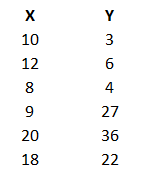
We will figure how to establish a relationship in this chapter and move closer towards the relative value trading technique. For convenience, let me post the table with the two number arrays once again –
| X | Y |
|---|---|
| 10 | 3 |
| 12 | 6 |
| 8 | 4 |
| 9 | 17 |
| 20 | 36 |
| 18 | 22 |
Clearly, casual eyeballing does not reveal any information about the relationship between the two sets of numbers. Maybe it does, if you are a mutant, but for a mere mortal like me, it does not work.

Under such circumstances, we rely upon a technique called the ‘Linear Regression’. Linear regression is a statistical operation wherein the input is an array of two sets of numbers and the output contains many different parameters, including the intercept and constant needed for constructing the straight line equation.
To perform the linear regression operation, we will depend on the good old Excel. Here is the step by step guide to perform a simple linear regression on two arrays of numbers. Be prepared to see a lot of screenshots and instructions ☺
Step 1 – Install the Plugin
Open a fresh excel sheet and insert the values of X & Y as seen in the above table. I’ve done the same as shown below –
This is our data set. Do remember, Y is the ‘Dependent’ variable whose value depends on the independent variable X. Both X and Y will be the input variables for the linear regression operation.
On the excel sheet, click on the Data ribbon as highlighted in red, shown below –
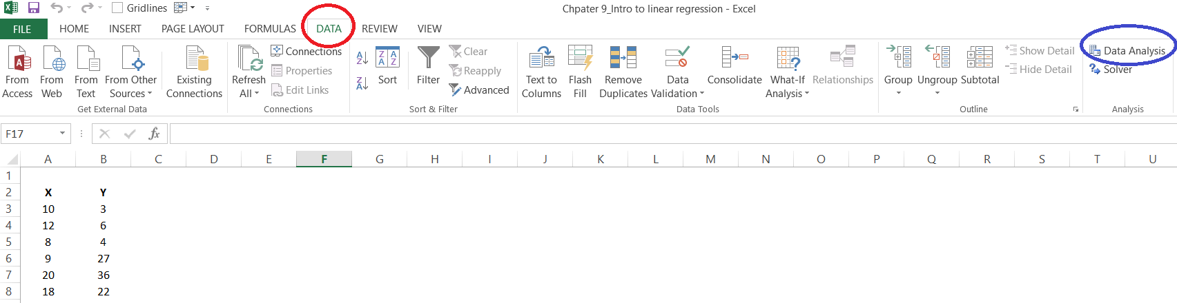
The data ribbon will now show you the ‘Data Analysis’, option. This is highlighted in blue. Now, some of you may not see this option, if yes, don’t panic. I’ll tell you what needs to be done.
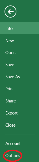
Click on ‘File’ –

This will open up a new window, and on your left-hand side panel, you will see an option to select ‘option’ –
Click on the Options, and you will see a bunch of general options to work with. On the left-hand panel, select ‘Add-Ins’, click on it and then click on the ‘Analysis Tool pack’. Then click on ‘Go’, and finally on ‘Ok’. With this, you’d essentially added the ‘Data Analysis’ option to the data ribbon.
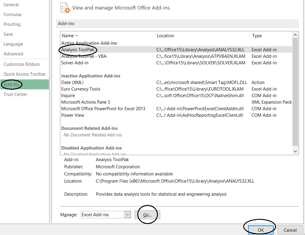
Close the excel sheet and restart your system and you are good to roll.
Step 2 – Enter the values
So we proceed further based on the assumption that your excel sheet has the data analysis pack. The next step is to invoke the linear regression function within the data analysis pack. To do this, click on the ‘Data’ ribbon, and select the Data Analysis. This will open up a pop-up, which will have a list of statistical operations which you can perform on data sets. Select the one which says ‘Regression’.
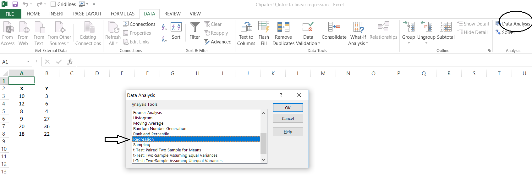
Select regression and click ok, you will see the following pop up –
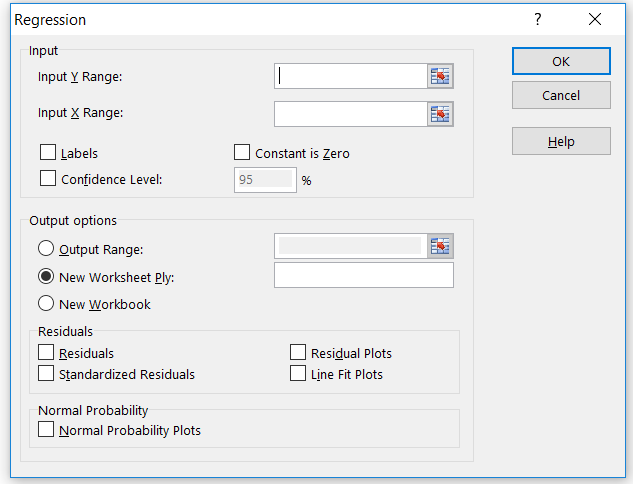
As you can see, there are a bunch of fields here. I’d suggest you pay attention to the first section, which is the input section. There are two fields here – ‘Input Y Range’ and ‘Input X Range’. As you may have imagined, Y is for the dependent variable and X is for the dependent variable.
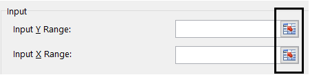
This is where we feed in the X and Y series data. To do that, click on the input channel and select Y and X range –
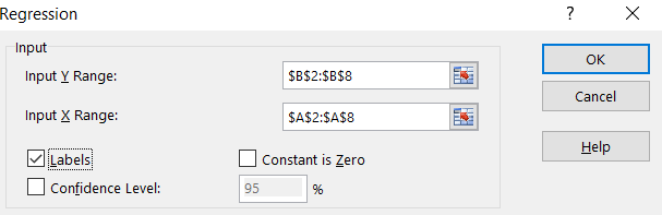
Also, please notice that I’ve checked the label box, this indicates that the first cell value i.e A2 and B2 contain the series label i.e X & Y respectively.
I’d suggest you ignore the other input values for now.
On the output side, ensure you’ve clicked the following –
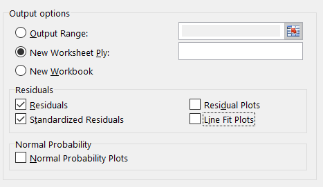
Selecting ‘New worksheet’, ensures that the output data is printed on a new worksheet. I’ve also clicked on two other variables called – Residuals and Standardized Residuals. I will talk about these two variables at a later point. For now, just ensure they are selected.
With this, you are good to perform the linear regression operation. Click on the ‘Ok’ button which is available in the right-hand top corner.
Excel will now take these inputs and perform the linear regression operation, the results will be posted in a new sheet within the same workbook.
9.2 – Linear Regression Output
So here is how the linear regression output looks and as expected, the summary of the output is presented in a new sheet.
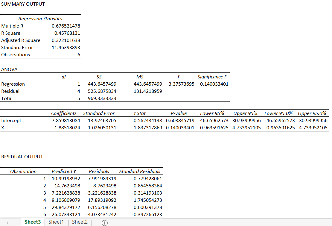
Agreed, the summary output is quite scary at the first glance. It has lots and lots of information. We will unravel this output in bits and pieces as we proceed.
For now, let’s concentrate on finding our slope and intercept. I’ve highlighted this for you in the below snapshot –
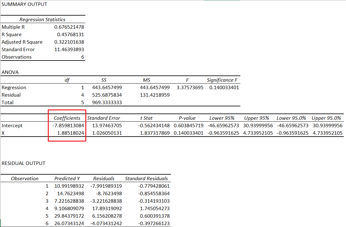
The data points highlighted in red contains the coefficients we are looking for i.e the intercept (or constant) and the slope (denoted by x).
Some of you may be confused with the slope being represented by x, I understand its misleading, it would have been best if it was M instead of x as it would match the straight-line equation, but then I guess we will have to live with x for slope.
So,
- Slope of the equation = 1.885
- Intercept (or constant) = -7.859813.
Given this, the straight-line equation for the arbitrary set of data is –
y = 1.885*x + (-7.859813) or
y = 1.885*x – 7.859813
So what does this really mean?
Well, if you recollect from the previous chapter, this equation essentially helps us predict the value of y or the dependent variable for a certain x. Let me repost the table here for the sake of convenience –
| X | Y |
| 10 | 3 |
| 12 | 6 |
| 8 | 4 |
| 9 | 17 |
| 20 | 36 |
| 18 | 22 |
| 15 | ?? |
I’ve added a new data point for x here i.e 15, now using the slope and intercept, we can predict the value of y. Let’s do that –
y = 1.885 * 15 – 7.859813
= 28.275 – 7.859813
= 20.415
So, if x is 15, then most likely, the predicted value of y is 20.415.
How accurate is this prediction, you may ask?
Well, it’s not accurate. It is only an estimation. For example, consider the value of x is 18 (refer to the last but one data point), then according to the straight line equation, the value of y should be –
y = 1.885*18 – 7.859813
= 33.93 – 7.859813
= 26.07019
However, the actual value of y is 22.
This leads us two values of y –
- Predicted value of y via the straight line equation
- Actual value of y
The difference between the two values of y is called the residuals. For example, the residual for y (difference between actual and predicted y), when x = 18 is
26.07019 – 22
= 4.070187
The summary output when you perform linear regression also contains the residuals, I’ve highlighted the same in the snapshot below –
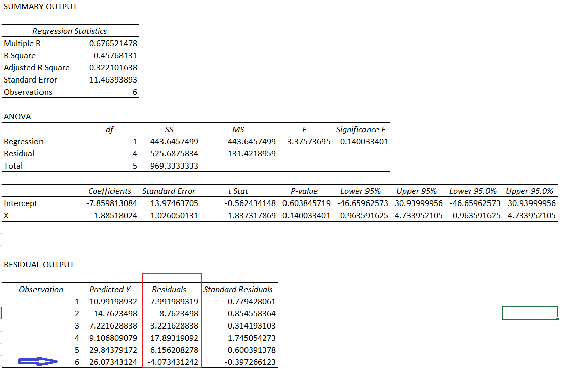
I’ve also highlighted the residual when x = 18, which is what we calculated above.
To give you a heads up – the bulk of the focus for carrying out the relative value trade depends on the residuals. Stay tuned!
Download the excel sheet here.
Key takeaways from this chapter
- Linear regression is a statistical operation which helps you construct a straight line equation
- Linear regression can be performed on excel. One needs to install the excel plugin to perform linear regression
- Amongst many other output variables, linear regression gives out the values of the slope and intercept
- With the help of the slope and intercept, one can predict the value of y
- The difference between actual y and predicted y is called the residual
- The residual is also a part of the output summary
taking x and y as two different stocks , these are daily returns we are calculating , right ? so if we know of x already , y has moved in the same time then what is the need to estimate?
I guess there is some typo:
So what does this really mean?
Well, if you recollect from the previous chapter, this equation essentially helps us predict the value of y or the dependent variable for a certain x. Let me repost the table here for the sake of convenience –
X Y
10 3
12 6
8 4
9 17
20 36
18 22
15 ??
: it should be 9 27
Ah, I need to double check this then.
In linear regression, after filling up the required data in input & output range,on clicking “OK”I’m. getting an alert that”input range must contain at least one data point “.What am I doing wrong? As in input Y range I have filled up”$B$2:$B$8” & in the row of input X range I have filled up”$A$2:$A$8”
Hiren, this is an excel error, not sure if I can help much on this. Usually, it helps to go step by step all over again.
the equation doesn<t satisfy the vaalues of x and y.Consider X=10 an Y=3.Now applying the equation you gave doesn't satisfy
Ah, why do you think so?
I think I wasn\’t clear, Sir. I didn\’t mean to ask whether you would use relative valuation in such situations. You have already answered that long back clearly. (Didn\’t mean to type repeated questions. Thanks for understanding)
I meant I would like to know which metric like \’P/E, EV/ EBITDA, Price to FCF\’ or something like that you would prefer to use \’the most\’ over the other. I\’m analyzing chemical sector, and using relative valuation seems like a challenge. I have no idea about which metric to prefer the most in this situation. Hence the confusion. Hope you got my question.
Ah, sorry, my bad, got that wrong. So each sector has sector-specific metrics which you should use. A few generic financial metrics that you mentioned will be the main bits in relative valuation, but apart, you also need to include sector-specific metrics. Like if you are looking at telecom, evaluating \’avg revenue per customer or ARPU\’, is relevant.
We have started covering each sector here – https://zerodha.com/varsity/module/sector-analysis/ , we will include chemicals soon.
I understand. But I meant, the relative valuation metric you prefer to you use the most in such situations?
Thats right, Sathish.
Sure sir. Thanks. In case you cant do DCF due to negative cash flow, what would be your preferred relative valuation metric you use the most?
Yeah, relative valuation works in such cases.
Sir, I came across the concept of regression in Mr.Aswath Damodar\’s book on valuation. Then took some efforts to get a brief idea and learnt about working it out on Excel sheets. Just now found this article. I understand this is about trading, but do you use linear or multiple regressions for valuation purposes. If yes, on what sort of situation do you use that? Thanks
Sathish, I\’ve never used regression in valuation, except probably while calculating a stock\’s beta. Have explained beta here – https://zerodha.com/varsity/chapter/hedging-futures/
do you know how to get the all the linear regression output data like excel in \”Google Sheets\” or \” in Numbers in Mac\” as I don\’t have excel and I am not able to find it in a proper way on the internet
Ah, not sure about this.
Hi Karthik,
I liked the this article. I\’ve one concern with the pair trading with linear regression. The assumption behind linear regression is that there should be linear relationship between Y and X. Why didn\’t you check it before building this model?
We do that step by step right?
Hi are the coeff you took statistically significant, if not can we still assume the coeff?
Linear regression line vs linear regression indicator
Hi Karthik
Thanks for great work. I have a quick question regarding Linear Regression. You have considered equation which has a constant however in case constant is negative, Y will have negative value for X at zero. Since this can not be possible, can we force equation to pass at origin and to get Beta only. And use this Beta for hedge ratio and subsequent calculations for residual calculations etc.
Thanks
Appy
Hmm, need to think through this. But I think it\’s hard to find pairs with a -ve constant. Did you find any?
Hi Karthik, indeed you are you are doing a great job by deciphering financial jargons for mango people of India. When read what you write it gives a classroom feel with a real friendly teach.
You have imparted me financial literacy right from module 1…I am thankful to you 🙂
Regards,
Rahul
So happy to note that, Rahul! Happy reading 🙂
Sir, we have not discussed the standardized residual in any of the chapters ahead. Is it not important at all?
If we have not, then probably it is not 🙂
hello Karthik sir,
Sir im not able to find the data analysis option as well as the file option please help
Varun, like I mentioned in the comments, we have put up only the sample files.
Hello Kartik,
This is really amazing to get so much information clearly and in laymen terms. Thank you for sharing information. Can I do an internship with you?
Regards,
Arihant Lodha
Arihant, glad you liked the content. Unfortunately, we don\’t have internship opportunities at Zerodha.
Respected KaRa Sir,
While i am reading up your articles on any topics, it is like you are reading my mind and making me understand things deeply.
Thanks for all your efforts.
Regards,
Chandan Chatterjee. 🙂
Thanks for the kind words and a new tag, Chandan 🙂
KaRa (khara) in Kannada means spicy 🙂
Keep learning and good luck !!
Can we do this in mobile?
It would be super cumbersome to do regression analysis on mobile 🙂
When is the PDF version of this entire chapter coming up?
Once the module is complete.
Sir is there any way to get the gauge the street sentiment of a particular stock or index.?
No tool as such, but you can feel it if you are glued in 🙂
Sir,
Can we estimate half life of pair with help of linear regression?
Thanks.
Hmm, I\’ll get back to you on this.
Karthik
First, Your work is truly appreciable. There is one query in my mind regarding Module-4, page no. 103-104, 10.3 calendar spreads. As in case you have taken positions in two contracts of different expiry of same underlying. While in box calculating P&L, You have taken only one expiry value for both contracts. How can price for contracts with different expiry will be same. Please help.
Shubham, I\’d suggest you keep track of module 10, which is work in progress. I\’ll be discussing a slightly better system to trade calendar spread.
Why residuals chapter is removed
Onkar, after posting the chapter I realized I\’ve made a mistake. I will rectify it and post it again next week.
Kartick,
you are simple one of the best educator I have come across during my professional life … Thanks for helping us.Eagerly waiting for cointegration module.
Regards,
Rajib.
Thanks for the kind words, Rajib 🙂
I\’m eager to write it as well!
Guruji,
You are going to write about co-integration….
I am eagerly waiting for it ….
This is all WOW….
Words OF Wisdom….
Pranam,
Arijit
I may touch that topic and stick to what really matters while trading, Arijit. Won\’t go too much into the details.
Guruji,
Basic is just good enough as I would be intetested in developing time series for index and options.
Thanks and Regards,
Arijit
Sure, I\’m yet to plan the outline. Mostly the discussion will be around something called as the ADF test. Will discuss this maybe in chapter 11.
Sir,
At what level u come to cointegration?
In maybe a chapter or 2, based on the flow.
Hello Karthik,
Are you going to explain any system that we could use in our daily basis?
If not, Please try to put out.
Thanks
Yes, I also plan to write about calendar spreads and delta hedging.
You have not mentioned about the use of linear regression.
Next chapter 🙂
Dear Karthik,
The sense that your articles are providing to understand the mindless market is quite great, I have never been fan of boring statistics 🙂 but the applications of the statistical methods here, has made me think differently. I guess this can be attributed to the real world application of statistics instead of the theoretical education that I was used to.
A stupendous work, I hope you continue to be a beacon for all of us.
Regards
Rajaram
P.S: I think there is a typo \”As you may have imagined, Y is for the dependent variable and X is for the dependent variable\”
Shouldn\’t X be the independent variable.
Thanks for the kind words, Rajaram. I\’m really happy to note that you\’ve liked the content here 🙂
Yes, that\’s a typo, will fix that, thanks for pointing out 🙂
Karthik – typo not fixed yet 🙂
Their is no downloadable link for module 10, please check that once.
Will be up once the module is completed.
Fantastic Karthik!!!
I eagerly wait for your new chapters like a school kid and check the varsity everyday. Hope to have the next chapter soon:)
Thanks for sharing the knowledge in such a lucid manner.
Thanks.
Happy to note that, Deepu 🙂 Motivates me to write more and faster 🙂
I have been waiting for it. Thanks:)
Happy learning 🙂
Can you develop charting tool to compare two stocks like techpaisa.com. Is there any other website
You can compare two stocks on Kite3, have you tried that yet?
comparing two stocks in kite? can you share a link how to do this? Just joined zerodha…Will be interested in knowing about this.
Comparing 2 scrips on Kite is explained in this TradingQ&A post
Thank you. i will search
Good luck!