5.1 – Deferred tax  

A gentleman posted an interesting comment in the previous chapter. The company he chooses to model did not present the gross block data in the way the company we are dealing with has, i.e. –

Gross block – Depreciation = Net block

Instead, the company directly reported the ‘Net block’ data.

Given this, how would one go about building the assumptions with Gross block as the base for many balance sheet based assumptions?

While the balance sheet reports only the ‘Net block’ number, the associated notes usually carry the gross block and depreciation numbers. One has to extract these details from the associated notes and rebuild the gross block.

It may sound a bit complex at this stage, but don’t worry; we will take this up in the next chapter and lay down the steps involved one at a time.

By the way, I hope you got to look at the raw data of P&L and Balance Sheet and layout the data in a model friendly manner. Assuming you’ve done that, we will now continue from where we left off in the previous chapter.

 

The previous chapter calculated the deferred tax’s growth rate from Y2 to Y5 and its average from Y6 to Y10. While this is ok, it still results in a somewhat volatile set of numbers. There is a better way to do this, and I’d like to discuss it.

If you understand deferred tax, you’d know that it occurs due to the way depreciation is treated. Hence deferred tax and depreciation is connected.

So, rather than taking the growth rate of deferred tax, it probably makes sense to consider deferred tax as a percentage of depreciation.

For Y2, the deferred tax is 16.95Cr, and depreciation is 121.73 Cr. So deferred tax as a percentage of depreciation for Y2 is –

16.95/121.73

= 13.92%

We can continue this for Y3, Y4, and Y5 on excel –

 

As you see, the numbers look much more stable. I’d request you to please make this change in your model. Now, for the projections, you need to take the rolling average. For Y6, it would be the rolling average of Y2 to Y5; for Y7, it’s the rolling average of Y3 to Y6 and likewise.

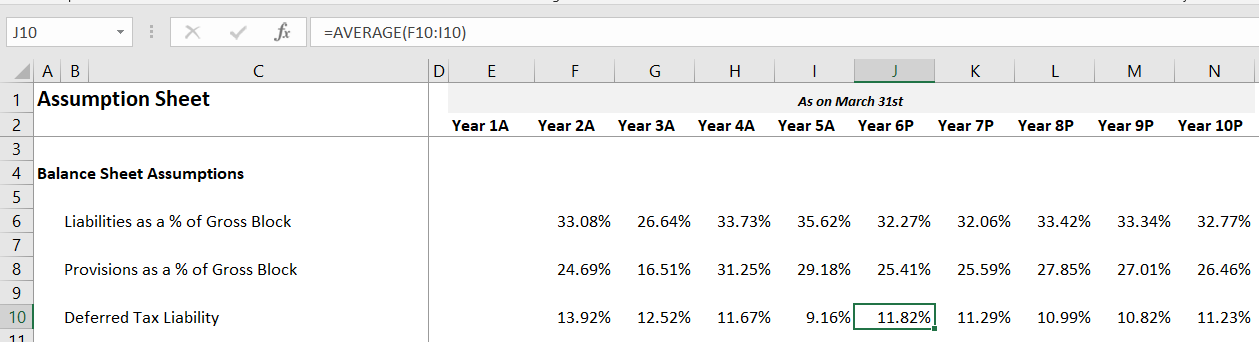
The resulting percentage range is also relatively stable.

Before you crib and curse me for making you redo the deferred tax bit, I’d like to tell you that the growth rate method for assumptions is critical, and we will use it in this chapter when we take up P&L assumptions.

So in that sense, you already have a heads up 😊

5.2 – Dealing with inventory 

With the deferred tax assumption, we also complete the liabilities side of the assumption. Please note that we have not made any assumptions for share capital and borrowings; these are line items we will deal with separately by building ‘schedules’.

So we now proceed to the asset side of the balance sheet, and the first line item to consider is the inventory.

If you look at the inventory data as stated in the balance sheet, you’ll realise the worth of inventory that’s lying with the company. For instance, for Y1, the inventory worth was 92.17 Crs; for Y2, it’s 194.33 Crs, Y3 it’s 160.83 Crs etc.

Any manufacturing company ends up having inventories in its balance sheet, and as you know, the inventory is nothing but the company’s finished goods. The objective of the company is to sell the inventory as quickly as possible. Hence lesser the number of days the company takes to sell the inventory, the better it is for the company.

Based on the nature of every company, the company takes up a certain number of days to convert its inventory to sales.

For example, a company manufacturing pressure cooker may convert its inventory to sales in 30 days, but a company manufacturing cars may take 75 days to convert inventory to sales.

When it comes to the inventory assumptions, we take the following approach –

• • • Convert the Rupee value of inventory to the number of days the company takes to convert to sales
    • Find the average number of days for the future years
    • Convert the average number of days back to the Rupee value for the future years

Sounds complex? Perhaps, but let’s go ahead and execute the above steps in our model and see how it goes. I’m sure you’ll eventually find it easy 😊

But before we proceed, why even take the pain of doing all the above? Why not directly take the growth rate of inventory and its average and move ahead (like how we treated deferred tax in the previous chapter)?

When you convert the Rupee value of inventory into the number of days to sales, you also get additional insights about the company. These insights help make investment decisions. For instance, imagine there are two companies manufacturing cameras that are similar in all aspects. Company A takes 40 days to convert inventory to sales, and company B takes 70 days to convert. What can you infer from this?

• • • Company A seem to have a better inventory management
    • Maybe Company A has a superior product. Hence the market prefer cameras from company A
    • Or maybe Company B’s sales incentives for merchants is not as attractive as A’s, so merchants tend to push Company A
    • Perhaps, company A have efficient management, meticulously planning these things

You see, the list of insights can go on and on. Hence it makes sense to take that extra effort to juggle and calculate the inventory number of days and let’s do that right away.

On excel, the inventory number of days is calculated easily by applying a formula. I call it the conversion formula because it converts the Rupee value of inventory to the inventory number of days.

For Y1 and Y2, the inventory value is 92.17 Crs and 194.33 Crs, respectively. To convert, we apply the following formula –

= (Average inventory of Y1 & Y2 / Materials consumed for Y2) * 365

In the denominator, you may ask why we use the materials consumed for Y2 and not Y1. Well, this is because we are calculating the inventory number of days for Y2. If we were to do this for Y1, then the formula is –

= (Average inventory of Y0 & Y1 / Materials consumed for Y1) * 365

Since we don’t have the Y0 data, we start with Y2.

So applying the formula for Y1 and Y2 –

= Average (92,17, 194.33)

= 143.25

Material consumed for Y2 (data available in P&L) = 762.86 Crs

=143.25/762.86

= 0.18778

Finally, we multiply the above result with 365 to get the inventory number of days –

= 0.18778 *365

= 68.53

The above number means the company takes about 68 days to convert 143.25Cr of inventory to sales.

Of course, you can do this in excel in one shot –

Please notice, I’ve included ‘inventory number of days in the assumption sheet and executed the conversion formula directly. I’d suggest you do the same in your excel.

Once I’ve calculated the inventory number of days for Y2, I can drag the excel to rows Y3, Y4, Y5 and get the respective values.

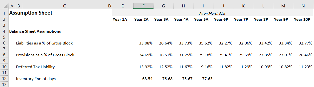
Notice, the inventory number of days consistently ranges between 68 to 78 days. To get a sense of how good or bad this number is, you need to compare it to a company operating in the same sector, of similar size. For example, Bajaj Auto and Hero Motors are similar companies doing similar business.

Moving ahead, for the Year 6 to Year 10, we can take the moving average of the inventory number of days.

We have calculated the historical inventory number of days and projected the inventory number of days for the future years.

In fact, you can take a similar approach to Sundry Debtor/Account receivables as well i.e. to convert receivables from Rupee value to receivable number days and then back to receivable in Rupee value.

In the next chapter, I’ll probably explain the process with the help of the helper model.

For now, let us move ahead with other balance sheets and P&L assumptions.

5.3 – Other Balance sheet assumptions

If you look at the asset side of the balance sheet, these are the line items stated by the company –

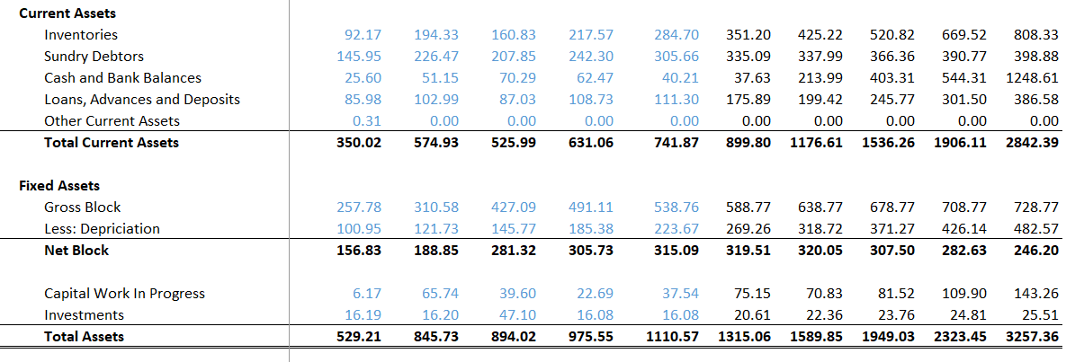
We have dealt with the inventories already.

Just like on the liabilities side, we will build a schedule for the gross block. Cash and Bank balance in current assets will be dealt with in detail in the cash flow statement.

We will make the assumptions for the remaining line items on the asset side. Let me quickly run you through the thought process before we jump to excel.

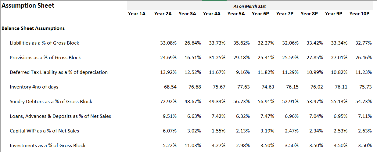
• • • Sundry debtors – I’ll consider this as a percentage of Gross block (but remember there is an alternate way i.e. to convert to days and back)
    • Loans, advances, and deposits – As you can imagine, this line item is related to the company’s working capital. Hence I’ll consider this as a percentage of net sales
    • Other current assets – This is a small number for Year 1 and does not exist for the rest of the years, so I’ll ignore
    • Capital work in progress – As a percentage of net sales
    • Investments – As a percentage of Gross block

Once I calculate the historical percentages, I’ll go ahead and calculate the rolling average for the future years. Like I’ve mentioned earlier, feel free to change the denominator based on your understanding of the firm and its financial statements. Remember, assumptions are the art bit in financial modelling; you are free to experiment, but ensure it is not too way out of wack 😊

So let me go ahead and implement the above in the excel sheet. I’ll post a series of snapshots hopefully that will be self-explanatory –

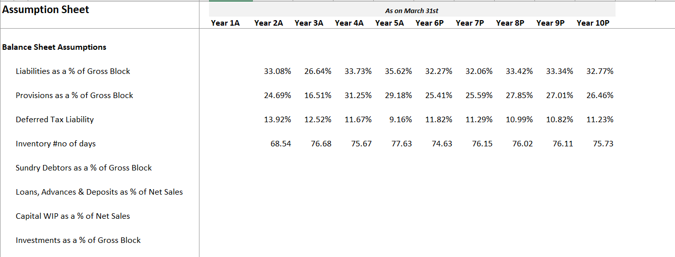
I’ve continued on the assumption sheet and lined up the line items in the same sequence as it appears in the balance sheet. Remember, I’ll do all the necessary calculations starting from Year 2 for consistency with the other assumptions.

I’ve calculated the percentages for Year 2, and I’ve highlighted the loans, advances, and deposits as a percentage of net sales. You can see both the formula bar as well as the F16 cell. I’ve highlighted this to showcases the  P&L line item in the denominator.

Hopefully, you will find this as an easy step to implement. Do let me know if you find any difficulties in implementing this by commenting below.

In the next step, I’ll drag the rows to the right till year five, and from year 6 onwards, I’ll take the averages.

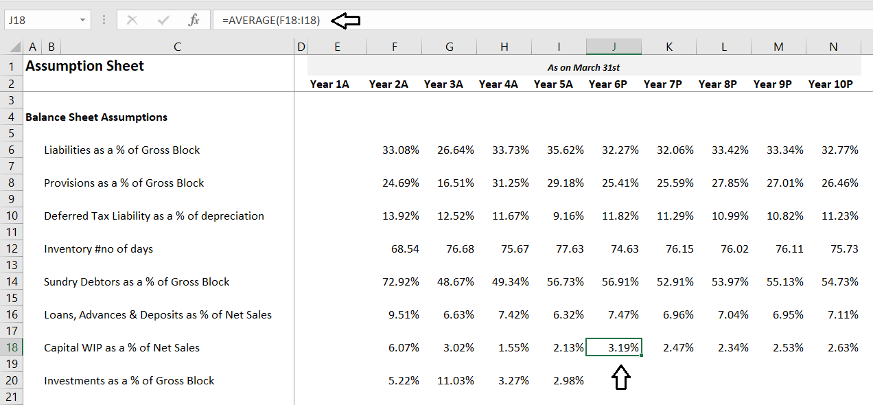
I’ve highlighted the average calculation for your better understanding. For the last balance sheet line item, i.e. investment as a percentage of Gross Block, I’ll not calculate the average for Y6 to Y10. Instead, I’ll assume a constant of 3.5% of the gross block.

Why not the average like other line items? Why 3.5%? Why not 4% or 3%? These are all valid questions.

The percentage calculated is quite volatile. It ranges from 3% to 11%, I’m not too happy with it, and therefore I’d like to keep it at a constant 3.5%.

Why not 4 or 3%? Well, that’s the beauty of a financial model. Once the model is complete, I can change this to any value that I think makes sense. Hence I don’t have to stress on it now and stick to 3.5% and move ahead.

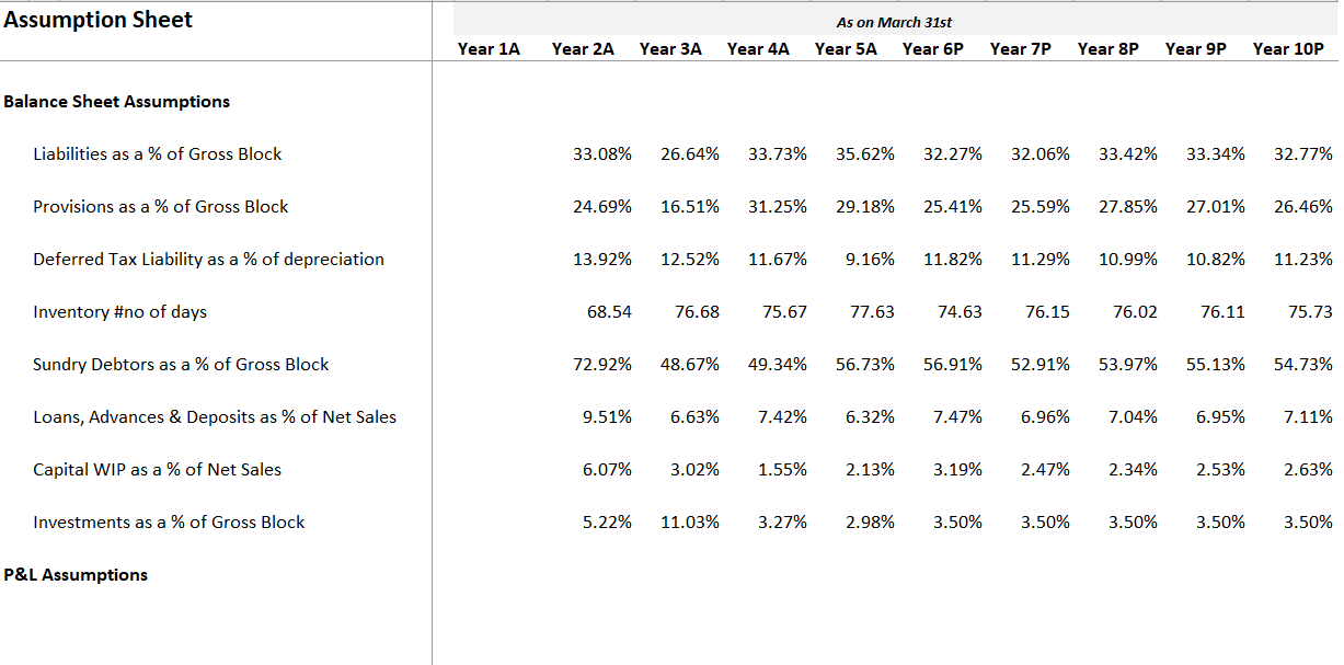
With this, we have completed the balance sheet side of assumptions. Whatever is left out will be dealt with in the form of schedules.

We will now move ahead with the P&L assumptions; this should be pretty easy.

5.3 – P&L assumptions

Let us start by taking a look at the P&L –

There is the revenue side, and then the expenses side to the P&L. Revenue side has the sales and other income data, while the expense has the details on all the expenses incurred during the year.

Making assumptions on the expenses side is super easy; all these line items are calculated as a percentage of the net sales or the total income. Revenues, on the other hand, is very interesting. You can either calculate the growth rate or deep dive to build a revenue model.

I want to discuss both these methods. In the primary model that we are dealing with, let us discuss the growth rate method of revenue forecasting. However, we will take the help of a helper model to build a revenue model.

Perhaps we can do both the revenue model and the receivable number of days in the next chapter.

Moving ahead, I’ll create another section in the assumption sheet to accommodate the P&L assumptions. Just for your clarity, this is how my assumption sheet looks at this stage –

Under the new P&L assumptions section, I will proceed sequentially, in the same order that the line items are present in the P&L.

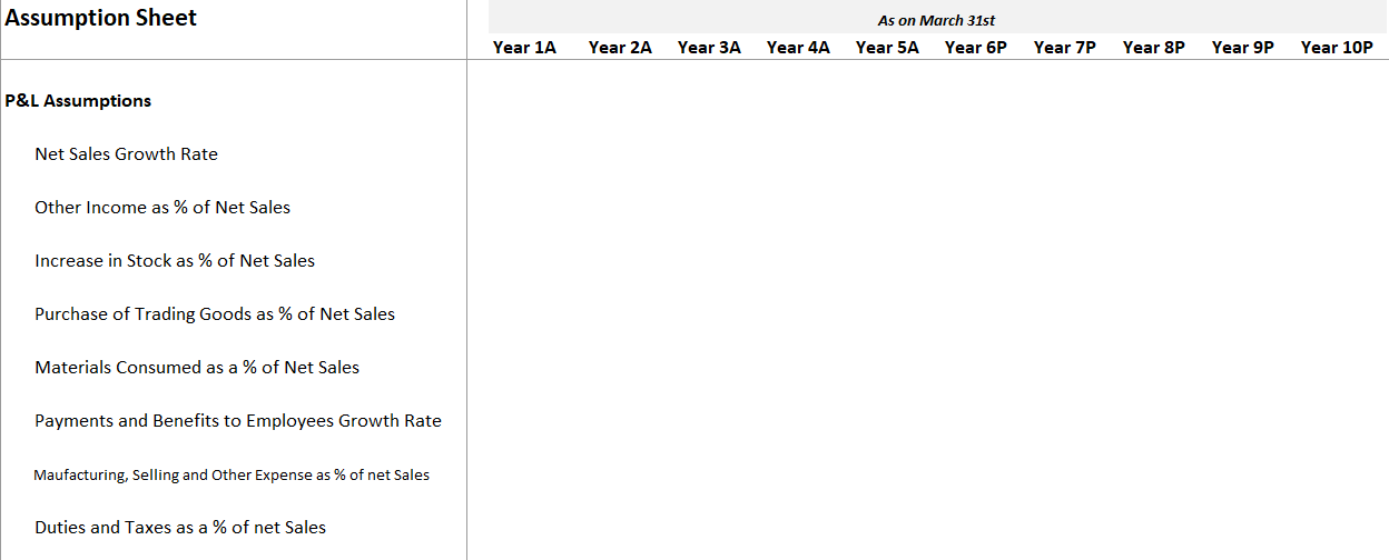
Notice, as discussed earlier, I’ve considered the growth rate for net sales, and for the remaining line items, I’ve considered these as a percentage of net sales. For example, other income is the percentage of the net sale; and the increase in stock is also a percentage of the net sale. So on.

Let us start with the Net sales growth rate; the growth rate is calculated the same way we calculated the deferred taxes growth rate in the previous chapter. Here is the snapshot of Net sales growth rate –

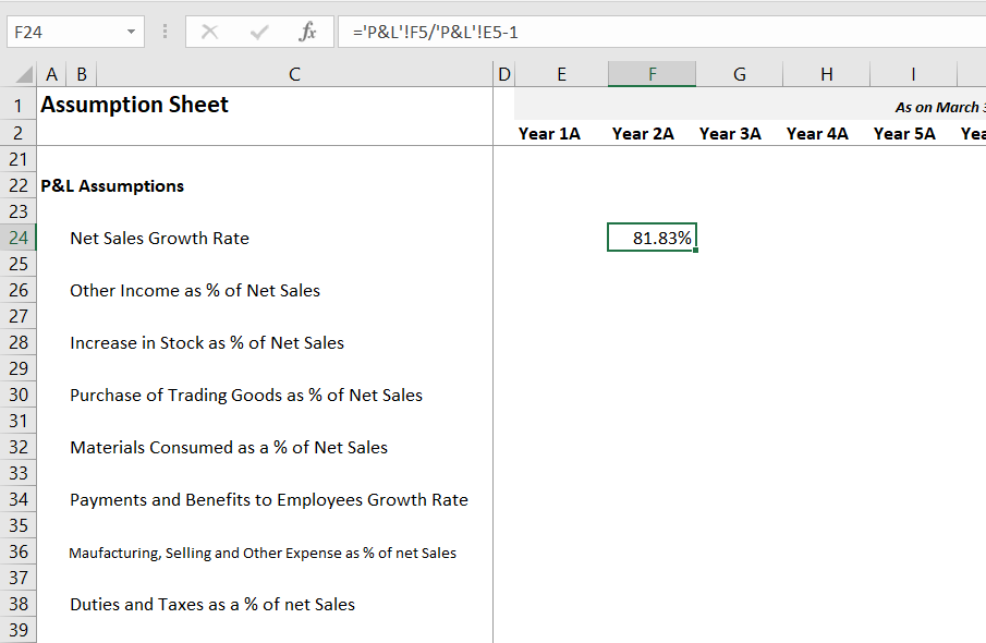
Yes, 81.83% seems high, but it is based on the net sales numbers reported by the company in Y1 and Y2. Here is something interesting that you can do. If you feel the numbers are unusually high, then you can always cross-reference how the peer companies performed during the same period.

If a company belonging to a particular sector has done phenomenally well for a particular year, its peer companies would most likely have performed equally well. For example, if MRF posts a 20% increase in revenue for Y1, you should expect Apolo Tyres to post a 20% increase in revenue. But for whatever reason, Apollo posts 16%, then you know that MRF probably has the edge over its competition.

Of course, this is a very rough example, but I’m highlighting this to give you a perspective of how you can think about companies while building the model.

I’ll go ahead and complete the P&L assumptions. As you can imagine, it is pretty straightforward, or so I assume because we have done this in the balance sheet assumptions.

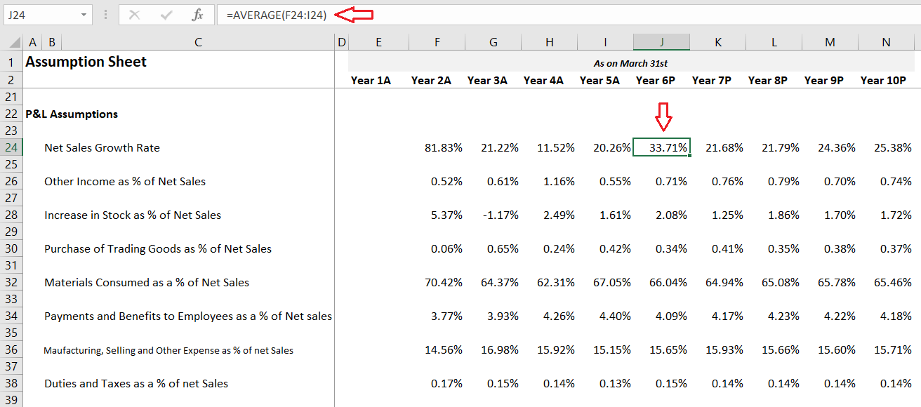
I’ve highlighted the Year 6 cell for net sales to showcase that subsequent calculations are all simple averages. Of course, this excel will be available for you to download and inspect each cell.

If you look at the P&L, the last two items on the expense side are Depreciation & Amortization and interest expense. These numbers will flow from the schedules that we will build subsequently.

The assumption sheet is now complete, and this is how it looks –

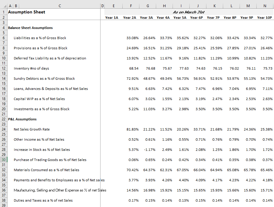
I’ve compressed the image to ensure you get to see the entire page.

I hope you followed the steps we’ve discussed in this and the previous chapter. Please do let me know if you have any queries; I’ll be happy to reply to your queries to the best of my abilities.

In the next chapter, we will take the help of a helper model and understand how to deal with receivables (assumptions) and set up a revenue model.

Download the excel sheet used in this chapter here.

Key takeaways from this chapter

• • • Deferred tax is as a percentage of depreciation
    • Converting inventory data from Rupee value to the number of days helps us develop unique perspectives into the functioning of the business
    • Likewise, with the Receivable data
    • A detailed revenue model gives granular insights into the revenue pattern of a company
    • All line items belonging to P&L and Balance sheet are assumed in the assumptions sheet. A schedule is built for the items which cant be assumed directly
    • Specific schedules give us granular insights into the specific line item