18.1 – Recap

We started chapter 1 with an introduction to financial modeling. I did talk about how financial modeling is always taught to students in a classroom program. An attempt to explain financial modeling in Varsity’s long-from approach was an interesting experience. The module took maximum planning and several rewrites, but I hope you recognize the complexity involved in this module 😊

As we approach the last chapter in this module, let us quickly recap everything we have learned so far in this module.

• As a first step, we discussed how to set up the excel sheet for building a financial model. We discussed format hygiene and how important it is to ensure cells are systematic across sheets. For example, column J represents Year 6’s data in sheet 1; then, we ensure column J is linked to year 6 data across all the sheets.
• We moved to import the historical data from the annual report. We copied mainly the P&L and Balance sheet statement. Just to let you know, there are multiple places where you can source these financial statements, including 3^rd party websites. But the best source for getting this information is the company’s annual report. So always try and stick to the annual report. We also color-coded assumptions and calculated numbers.
• We set up an assumption sheet, where we dumped all the assumptions on one page. The page itself is divided into P&L assumptions and Balance sheet assumptions. We discussed two techniques of assumption – the growth driver by taking historical averages and the percentage technique.
• For some companies having a dedicated revenue model helps. A revenue model gives us granular insights into things that can impact the company’s revenue.
• We built the asset and debt schedule of the company. Asset schedule gives us insights into depreciation and CAPEX. The debt schedule gives us insights into the cost of debt. Both these sheets link back to the balance sheet.
• The Reserve schedule is another schedule we built, with numbers from both P&L and balance sheet.
• With all the schedules and assumptions in place, we make P&L and Balance sheet projections. At this stage, all the line items in the P&L and Balance sheet get projected. What remains are the cash and cash balance numbers on the balance sheet.
• We built the cash flow statement using an indirect method to get the cash balance. The final cash value flows back to the balance sheet, and if the calculations are correct, the balance sheet should balance at this stage.
• The financial model is said to have hit a milestone when the cash value hits the balance sheet to balance the balance sheet.
• After the cash flow statement chapter, we discussed the theory of valuations, and now, it is time to implement the valuation model and bring all the concepts together.

Over the last few chapters, mainly from chapters 14 to 17, we discussed theoretical concepts related to valuation. In this chapter, let us implement the discounted cash flow valuation (DCF) model within the primary model. The output from the DCF model is the share price of the company.

18.2 – Assumptions

From a format perspective, the DCF model sheet will look a bit different from the rest of the model sheets because we are not dealing with any historical data. However, as usual, we will start by indexing columns A and B and rename the sheet to ‘DCF valuation.’

To begin with, we will dump all the data we need to implement DCF.

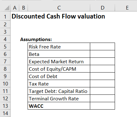
I hope you’ve read the previous few chapters so that these terms don’t suddenly look alien to you 😊

• We can use the long-dated Govt securities (bond) yield as a proxy for the risk-free rate. The data is available for you on RBI’s website. As of today, I’ll take the 10-year bond’s yield as a proxy, which is at 7%
• The beta of the stock is pretty easy to calculate. I’ve explained it in this chapter here. Refer to section 11.5. I’ll assume the beta of the company we are modeling as 1.2. As you may know, a beta of 1.2 is high beta. But don’t worry; you can change these numbers anytime since this is an integrated financial model.
• The expected market return is the standard market expectation and can range between 10% and 12%. Let us go with 12% for now.
• The cost of Equity is derived from the CAPM formula discussed in the previous chapters. It is the risk-free rate plus the difference between the expected market rate and the risk-free rate multiplied by the company’s beta. It is easy if you look at the excel formula.
• The cost of debt is the rate at which the company borrows funds—assuming this to be 10%.
• The tax rate is 25%. Of course, you can change this to any percentage you think makes sense.
• The target debt-to-equity ratio is assumed to be 50%. While it’s nice to be debt-free, most companies cannot afford to be. They do end up taking debt to fund CAPEX, but a well-run company will aim not to cross the 50% threshold.
• The terminal growth rate is a super important assumption that we make. The entire DCF model relies heavily on this assumption. As discussed in the previous chapter, we will assume the terminal growth rate to be close to the long-term inflation number of the country, so between 4 and 5%.
• The weighted average cost of capital (WACC) is something that we will calculate in excel directly. But I do hope you recollect the discussion we had previously on WACC.

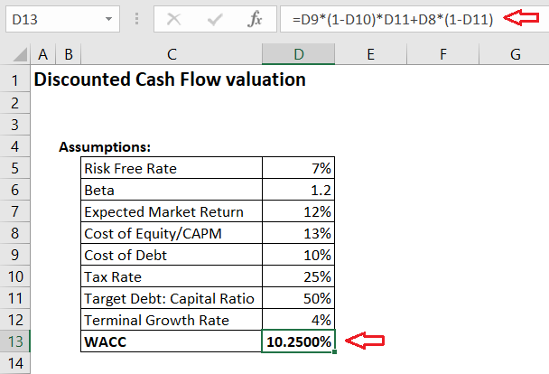
WACC is the weighted average return expectation of debt holders and equity holders (check highlights). We will use the WACC to discount the cash flows.

18.3 – Free cash flow to the Firm

Once we have the assumptions in place, we have to calculate the free cash flow to the Firm (FCFF). Remember, we are calculating the future free cash flows to the Firm. Hence we have to deal only with data from year six onwards. We start the calculation with EBIT and take the tax shield effect on EBIT.

Of course, we have not calculated EBIT specifically in P&L, so we will have to quickly figure that in P&L. EBIT is earnings before interest and taxes; hence to calculate EBIT, we subtract all the expenses from total income, except the interest.

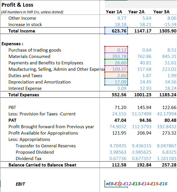
We multiply EBIT with (1-tax rate) to factor in the tax shield effect on EBIT. To this, we add back all the non-cash charges and deduct working capital and CAPEX charges to arrive at the free cash flow to the Firm. I’ve made these calculations in excel, and here is how my sheet looks now –

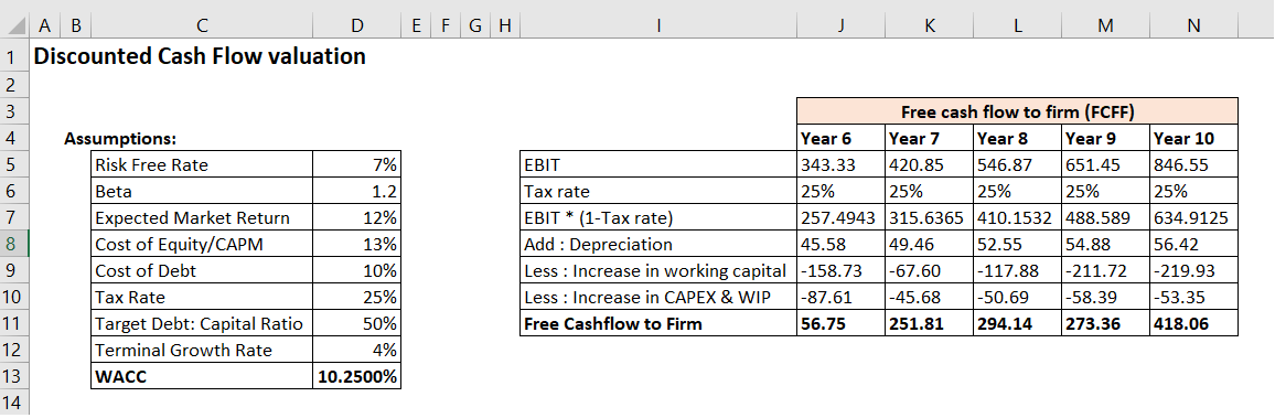
Notice that I’ve indexed columns E,F,G, and H to ensure I link columns J to N with years 6 to 10, just like in the other sheets. You are free to format this sheet in whatever way you think makes sense.

EBIT and depreciation numbers come from P&L. The working capital and CAPEX numbers come from the cash flow statement. I’ll provide the link to download the excel sheet at the end of this chapter, so please do download the sheet and check the cell linkages.

18.4 – Terminal Growth value

We now have the free cash flow to the Firm, projected up until the next five years, i.e., till year 10. However, this does not mean the company will stop generating free cash flow after five years. We assume that the company will not only continue to exist but will also continue to generate free cash flow. The rate at which the cash flow grows is called the ‘terminal growth rate,’ which is usually equivalent to the long-term inflation value of the country.

I want you to use a bit of imagination here. Fast forward to 5 years from now. From the 5^th year onwards, you are looking outwards at eternity and imagining all cashflows that the company will generate. You need to sum up all the cash flow and bring it to the 5^th year, i.e., the current year.

You can do this by applying the terminal growth value formula –

= 5^th Year cash flow * (1+terminal growth rate)/(WACC-terminal growth rate)

I’ll not get into the technicalities of how the formula is derived. But that’s the formula to figure out the sum of all the future cash flows.

Here is the calculated value –

The terminal value is a big number and has an impact on the final valuation of the company.

So, we have the next five year’s free cash flow to the firm numbers. We also have the terminal value number. We now have to discount all these cash flows and bring them back to the present-day terms, i.e., we need to calculate the present value of all the future cash flows.

For example, the free cash flow in Year 8 is 294.14 Crs. Year 8 is three years away from the present day. To calculate the present value –

= 294.14/(1+10.25%)^3

= 219.4923 Crs.

We can do this systematically in excel –

I first calculated something called a discount factor, which is –

1/(1+WACC)^(time)

The time for this particular example is three years. So the discount factor for year 3 is 0.746. I have to multiply the discount factor with the free cash flow to get the present value.

So 0.746 * 294.14 = 219.4923Crs.

Notice that I’ve also calculated the present value of the terminal growth value.

18.5 – Share price

We’ve come to the last bit, finally 😊

We sum up all the present value of the future free cash flow, i.e., from Year 6 to 10, along with the current value of the terminal value to arrive at the ‘Enterprise Value. We deduct the present-day debt from the enterprise value and add the present-day cash to give equity holders the free cash flow.

The present-day debt and cash value come from the balance sheet.

And, here you go –

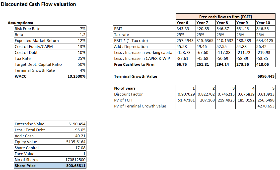
The share price is Rs.300. What does this mean?

The price you see here is an outcome of the entire valuation exercise. We have made many assumptions here, and if these assumptions are made intelligently, then with some confidence, we can conclude that Rs.300 is the fair value of the stock. You can now compare the stock’s market value on the stock exchanges and decide to buy or wait. For example, if the stock is trading at Rs.425, then you know that it is overvalued compared to its fair value; hence you can avoid buying the stock.

If the stock is trading at Rs.225, the stock is undervalued, and you can go ahead and invest in the stock. Or if the stock is trading at Rs.300, it is said that it is fairly valued.

18.6 – Closing thoughts

The model we have built is integrated, meaning that any change in any number in this model will impact the share price.

For example, in the assumption sheet, I’ll change the material consumed as a percentage of sales for Year 6 to 60% from 65%. The share price will change to Rs.462 from Rs.300.

Or I can change the terminal growth rate to 4.5% from 4%, and subsequently, the share price changes to Rs.323. I encourage you to make these changes and see for yourself, which is the beauty of this model. All the sheets and numbers are linked, and any difference across the sheet will result in the final output.

You can make these changes when you think the difference is justified, which brings me to my next point.

Building a financial model is pretty straightforward. A seasoned modeler will probably create a good model in a few days. But what is essential is to keep the model up to date. Once you build a model, track the company closely, especially the management interviews and statements. Whenever new information comes, make an appropriate change in the model.

For example, during the following quarterly result announcement, the company may say they want to slow down their CAPEX spending. Immediately, tweak your model and adjust for a lower CAPEX spend, and accordingly, the share price changes and gets re-rated. Maintain a separate sheet in the workbook detailing the reasons based on which you made the changes. The sheet acts as your working notes.

One last thing before I end this chapter and module – the final output, i.e., the share price is Rs.300. That does not mean, Rs.300 is strictly the fair value of the stock. The share price is an output of a model we have built, and the model is undoubtedly prone to inadvertent errors. Therefore, you need to factor in model errors. I’d assign a 10% band as a modeling error, which means I’ll consider the stock’s fair price anywhere between Rs.270 to Rs.330.

I’ll be happy to buy the stock anywhere within this range, preferably at the lower end, as it gives me some margin of safety.

I hope you enjoyed reading through this module as much as I enjoyed writing this for you.

You can download the excel sheet from here.

Key takeaways from this chapter

• The stock’s beta represents the stock’s riskiness with respect to the market and can be easily calculated.
• We use the CAPM equation to figure out the cost of equity
• WACC is a blended cost of capital that we use to discount the cash flow
• Free cash flow to the Firm is calculated by starting with EBIT
• You can calculate the discount factor to calculate the present value easily
• Enterprise value is the sum of all the present value of future cash flow
• As and when new information flows, one needs to update the model
• The final share price is just an indicator of fair value. It makes sense to factor in model errors and assumes a fair value price band rather than a since price as the fair value of a stock.