4.1 – Model integrity

I want to start this chapter by talking about a super important concept. I may have touched upon this topic earlier, but I would like to discuss it again with snapshots to emphasise its importance.

In the previous chapter, we set up the balance sheet and P&L for the helper model. Here is the snapshot of the same –

P&L –

And the balance sheet –

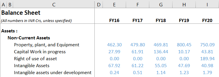
The model design ensures column E represent FY16 data, column F to FY17 so on and so forth. We do this to ensure that the numbers get identified quickly and linkages between cells are accurate.

For example, imagine a scenario wherein I want to calculate the ratio of Property, plant, and equipment to the Total revenue for FY18. If you realize, to calculate this, I need to divide a balance sheet item with a P&L item, which means I will have to crisscross between sheets to do the math. This further means that I can easily link the wrong cells without evening noticing it.

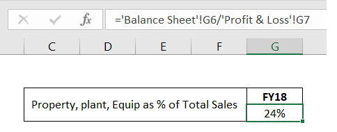
Anyway, let us go ahead and do this. I can easily calculate by linking the cells of Column G in the formula bar –

Now consider a situation where you’ve linked the wrong years while calculating this ratio. You can spot the wrong linkage easily –

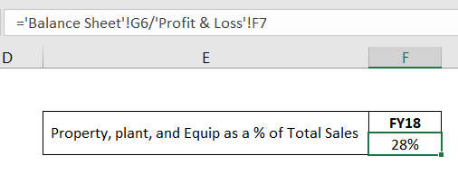
In this case, I know column G in the balance sheet should be linked with column G of P&L. The moment I see the G and F combination, I know something is wrong.

I’ve quoted a relatively simple example here. But as the model grows and gets more complex, you’ll understand and appreciate the need to maintain the model integrity.

4.2 – Main model

It’s time to introduce you to the primary model. I’m sure many of you here would expect me to name the company we’d work on and also name the years under consideration. But I have different plans 😊

I’d rather keep the name and years under consideration unknown. I’m doing this for two reasons –

• By not naming the company, I’ll hopefully eliminate biases one may have. For example, if I use a footwear manufacturing company’s data, some may feel that it may not apply to an auto component company. So I think it is better to keep it generic to establish the fact that this model template applies to all companies (except banking and NBFC)
• Hopefully, by not quoting years, someone reading this module five years later will also understand that the overall structure of a financial model remains the same, no matter when you decide to learn financial modelling.

But for the sake of your understanding, assume that we are dealing with a simple manufacturing company’s data.

I’ve used the exact steps detailed in the previous chapter and set up the Balance Sheet and P&L data. Here is the snapshot of the same –

Balance sheet –

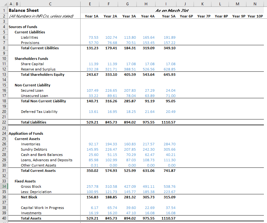
I’ve shrunk my excel sheet to 70% to ensure I capture both sides of the balance sheet; hence the numbers and format look a little different.

Here is the snapshot of the P&L –

A couple of things here –

• • The years in consideration is Year 1, Year 2, Year 3 up to year 5 etc. It means the latest 5 years of data. So even if you read this 10 years later, it won’t matter.
  • The data is from the Annual Report, as of March 31^st,e. the financial year-end
  • Year 1A means Year 1 actual data. Year 6P means the year 6 data projected. The projected data is also as per March 31^st. In a sense, this is our vision of how the financial statement will look like future annual reports

You can download the excel sheet from the end of this chapter. In the excel sheet, you’ll find the raw P&L and Balance sheet data; I’d suggest you use that data and lay it down in the format we’ve discussed. It will be good practice for you.

4.3 – Assumptions and Projections

Remember, in the first chapter; I mentioned that financial modelling is a bit of art and financial science?

The art part starts now 😊  

The idea behind a financial model, quite obviously, is to analyse the historical financial statements and project them forward. The common practice is to project the number to either three or five years forward. In this model, we will try and deal with five years projections.

To get an initial understanding of this, I’ll post a set of questions and answers –

>>>> How will you project the financial statements for the future years?

>>>> Well, you can project the financial statements by making a set of assumptions.

>>>> How will you assume these things to help you make the necessary projections?

>>>> We can assume the future trends based on historical trends.

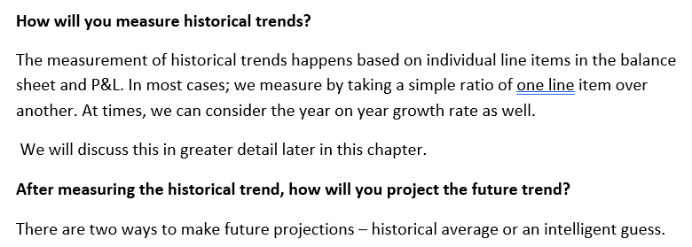
>>>> How will you measure historical trends?

>>>>> The measurement of historical trends happens based on individual line items in the balance sheet and P&L. In most cases; we measure by taking a simple ratio of one line item over another. At times, we can consider the year on year growth rate as well.

 We will discuss this in greater detail later in this chapter.

>>>> After measuring the historical trend, how will you project the future trend?

>>>> There are two ways to make future projections – historical average or an intelligent guess.

At this point, I just want you to read the above and keep this in the back of your mind. Some parts may be clear, and some parts may sound confusing, but I hope by the end of this chapter, you’ll get a clear understanding of this topic.

With that in mind, let us go ahead and make our first assumption for the financial model, but before that, let’s set up our assumption sheet.

To set up the assumption sheet, please go to a new sheet in the workbook and rename the sheet to ‘Assumption’ at the bottom.

Now, we do the usual, i.e. –

1. Index column A and B
2. Expand column C
3. Index column D
4. Cells E2 to I2 will be Year 1 to Year 5
5. Cells J2 to N2 will be Year 5P to tear 10P

I’ve followed the same steps, and here is how my excel sheet now looks.

The idea with the assumption sheet is to lay down each of the financial statements line items and project it based on our assumptions. So let us go ahead and lay down these line items. Let me start with the Balance sheet; take a look at these two lines in the balance sheet, i.e. liabilities and provisions under the current liabilities section –

Now, recollect this part from the QnA we had earlier –

To measure historical trends, we usually take the line item as a ratio of another line item. For the balance sheet, usually, the ratio is measured by keeping the ‘Gross Block’ as the denominator. Gross block, because the gross block is one of the most oversized balance sheet items, also sucks up the company’s CAPEX.

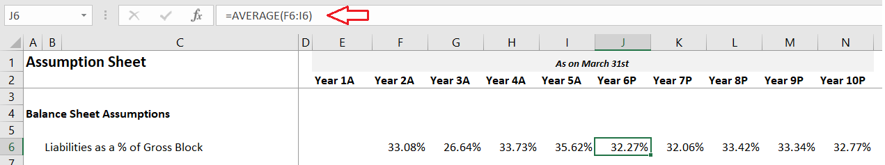
So, if you were to look at ‘Year 2’, liabilities as a percentage of Gross block,

Liabilities as a % of Gross Block (Y2) = 102.74/310.58

= 33.08%

Of course, we can do this in excel directly –

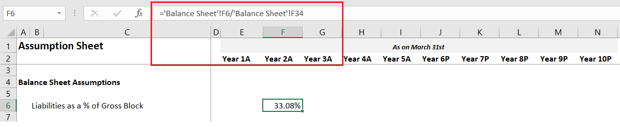
Notice, I’m dealing with Year 2 data. Hence in the balance sheet, I divide F6 over F34.

You may wonder why I’ve done this for Year 2 and not for Year 1. This is because there will be instances where we’d need to calculate the year-on-year growth rate, which means our starting point will be year 2. Hence, for this reason, we ignore Year 1 and directly deal with year 2. You will notice this pattern in several places throughout this module.

Alright, now that we have calculated  Liabilities as a % of Gross Block, we can drag the formula across Y3, Y4, and Y5.

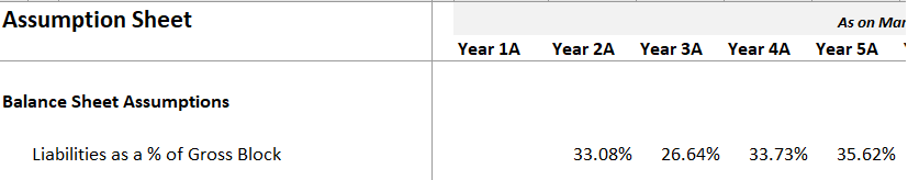
As you can see, liabilities as a percentage of gross blow hovers between 27% and 35% consistently. So, if I were to figure out what this ratio would be for Year 6, I can just take the historical average and get a perspective.

Let me do the same –

Congratulations! With this, we have projected the very first line item of our balance sheet. Few things to note here –

• • I’ve used the simple average function here
  • The first average, i.e. for the year 6, is the average of Year 2 to Year 5
  • The 2^nd average, i.e. for year 7, the average is between Year 3 and Year 6
  • We are calculating the rolling average here, so at any point, we consider the latest four years data
  • The average which we have calculated hovers within the expected range, i.e. between 27% and 35%, so this is ok.

Whenever you calculate such ratios, it is best if the variance range is narrow. The narrower the range, the more consistent is the average calculation. The more consistent the average, the tighter is your model.

I’m not too happy with a range, i.e. 27% to 35%; it could have been better. If you are not too happy with it, you can try exploring other ratios like ‘labilities as a percentage of total assets or as a percentage of netblock or something like that.

Wait! So what should you consider? Liabilities as a % of the gross block, or netblock, or total assets?

Well, this is where the art form kicks in. There is no guiding principle here. There is no rule which says you have to consider the denominator as gross block only. I’ve taken it because I’m comfortable with it.

The end objective here is to ensure the calculated numbers are as consistent as possible. Also, don’t stress too much on this; after all, this is a financial model based on excel. We can change things at any point during this journey.

I’ll now go to the next line item, i.e. the Provisions under the current liabilities. Again, I’ll calculate provisions as a percentage of the gross block.

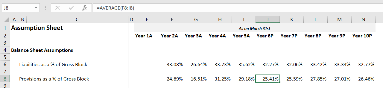
Hopefully, you get the drift by now.

Let us go back to the balance sheet for a bit –

Under the liabilities side, we have projected Provisions and Liabilities. What’s next is shareholders funds and non-current liabilities. Usually, big-ticket items like these in the balance sheet should be dealt with separately in the financial model. We deal with it by creating something called a ‘Schedule’. Of course, we will talk more about schedules later in the module, but for now, think about schedules as a separate dedicated sheet within the financial model.

So all the things marked is treated in the schedule, where we will also make future projections. That leaves us with just the deferred tax liabilities on the liabilities side of the balance sheet.

For the deferred tax liabilities, I’ll consider the year on year growth rate. If you look at Y1 and Y2 numbers, it’s at 13.61 Cr and 16.95Cr. To calculate the year on year growth rate –

(16.95/13.61) – 1

= 25.55%

Note, this is the growth rate for Year 2. On excel –

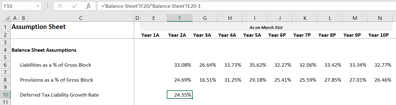
Of course, you can now drag the cells for the rest of the years, up to Year 5, and take the rolling average from Year 6 onwards.

We now move to the asset side of the balance sheet. Perhaps, I’ll take it up on the next chapter, and I promise I’ll put up the next chapter soon 😊

You can download the excel sheet used in this chapter from here; please note, this excel also includes the raw data. I’d encourage you to use the raw data and build the P&L and Balance sheet from scratch.

 Key takeaways from this chapter

• Please pay attention to model integrity, as it helps you identify accurate cell linkages
• One can calculate the historical trends either as a growth rate or by taking a simple ratio
• Projections are made by taking averages or by making an intelligent guess
• It is best when the historical trends exhibit a non-volatile range
• Assumptions are an art form; there is no standard method to make assumptions. Your guess is as good as mine.