10.1 – Black Monday
Let’s start this chapter with a flashback. For many of us, when we think of the 70’s, we can mostly relate to all the great rock and roll music being produced from across the globe. However, the economists and bankers saw the 70’s very differently.
The global energy crisis of 70’s had drawn the United States of America into an economic depression of sorts. This lead to a high inflationary environment in the United States followed by elevated levels of unemployment (perhaps why many took to music and produced great music 🙂 ). It was only towards the late 70’s that things started to improve again and the economy started to look up. The Unites States did the right things and took the right steps to ease the economy, and as a result starting late seventies / early eighties the economy of United States was back on track. Naturally, as the economy flourished, so did the stock markets.
Markets rallied continuously starting from the early 1980s all the way to mid-1987. Traders describe this as one of the dream bull runs in the United Sates. Dow made an all-time high of 2,722 during August 1987. This was roughly a 44% return over 1986. However, around the same time, there were again signs of a stagnating economy. In economic parlance, this is referred to as ‘soft landing’ of the economy, where the economy kind of takes a breather. Post-August 1987’s peak, the market started to take a breather. The months of Aug, Sept, Oct 1987, saw an unprecedented amount of mixed emotions. At every small correction, new leveraged long positions were taken. At the same time, there was a great deal of unwinding of positions as well. Naturally, the markets neither rallied nor corrected.
While this was panning on the domestic front, trouble was brewing offshore with Iran bombing American super tankers stationed near Kuwait’s oil port. The month of October 1987, was one of its kind in the history of financial markets. I find the sequence of events which occurred during the 2nd week of October 1987 extremely intriguing, there were way too much drama and horror panning out across the globe –
- 14th Oct 1987 (Wednesday) – Dow dropped nearly 4%, this was a record drop during that period
- 15th Oct 1987 (Thursday) – Dow dropped another 2.5%. Dow was nearly 12% down from the August 1987’s high. On the other side of the globe, Iran attacked an American super tanker stationed outside Kuwait’s oil port, with a Silkworm missile
- With these two events, there were enough fear and panic spread across the global financial markets
- 16th Oct 1987 (Friday) – London was engulfed by an unexpected giant storm, winds blowing at 175 KMPH caused blackouts in London (especially the southern part, which is the financial hub). London markets were officially closed. Dow opened weak, and crashed nearly 5%, creating a global concern. Treasury Secretary was recorded stating economic concerns. Naturally, this would add more panic
- 19th Oct 1987 (Black Monday) – Starting from the Hong Kong, markets shaved off points like melting cheese. Panic spread to London, and then finally to the US. Dow recorded the highest ever fall with close 508 or 22.61% getting knocked off on a single day, quite naturally attracting the Black Monday tile.
The financial world had not witnessed such dramatic turn of events. This was perhaps the very first few ‘Black Swan’ events to hit word hard. When the dust settled, a new breed of traders occupied Wall Street, they called themselves, “The Quants”.

10.2 – The rise of quants
The dramatic chain of events of October 1987 had multiple repercussion across the financial markets. Financial regulators were even more concerned about system wide shocks and firm’s capability to assess risk. Financial firms were evaluating the probability of a ‘firm-wide survival’ if things of such catastrophic magnitude were to shake up the financial system once again. After all, the theory suggested that ‘October 1987’ had a very slim chance to occur, but it did.
It is very typical for financial firms to take up speculative trading positions across geographies, across varied counterparties, across varied assets and structured assets. Naturally, assessing risk at such level gets nothing short of a nightmarish task. However, this was exactly what the business required. They needed to know how much they would stand to lose, if October 1987 were to repeat. The new breed of traders and risk mangers calling themselves ‘Quants’, developed highly sophisticated mathematical models to monitor positions and evaluate risk level on a real-time basis. These folks came in with doctorates from different backgrounds – statisticians, physicist, mathematicians, and of course traditional finance. Firms officially recognized ‘Risk management’ as an important layer in the system, and risk management teams were inducted in the ‘middle office’ segment, across the banks and trading firms on Wall Street. They were all working towards the common cause of assessing risk.
Then CEO of JP Morgan Mr.Dennis Weatherstone, commissioned the famous ‘4:15 PM’ report. A one-page report which gave him a good sense of the combined risk at the firm-wide level. This report was expected at his desk every day 4:15 PM, just 15 minutes past market close. The report became so popular (and essential) that JP Morgan published the methodology and started providing the necessary underlying parameters to other banks. Eventually, JP Morgan, spun off this team and created an independent company, which goes by the name ‘The Risk Metrics Group’, which was later acquired by the MSCI group.
The report essentially contained what is called as the ‘Value at Risk’ (VaR), a metric which gives you a sense of the worst case loss, if the most unimaginable were to occur tomorrow morning.
The focus of this chapter is just that. We will discuss Value at Risk, for your portfolio.
10.3 – Normal Distribution
At the core of Value at Risk (VaR) approach, lies the concept of normal distribution. We have touched upon this topic several times across multiple modules in Varsity. For this reason, I will not get into explaining normal distribution at this stage. I’ll just assume you know what we are talking about. The Value at Risk concept that we are about to discuss is a ‘quick and dirty’ approach to estimating the portfolio VaR. I’ve been using this for a few years now, and trust me it just works fine for a simple ”buy and hold’ equity portfolio.
In simple words, Portfolio VaR helps us answer the following questions –
- If a black swan event were to occur tomorrow morning, then what is the worst case portfolio loss?
- What is the probability associated with the worst case loss?
Portfolio VaR helps us identify this. The steps involved in calculating portfolio VaR are very simple, and is as stated below –
- Identify the distribution of the portfolio returns
- Map the distribution – idea here to check if the portfolio returns are ‘Normally distributed’
- Arrange portfolio returns from ascending to descending order
- Observe out the last 95% observation
- The least value within the last 95% is the portfolio VaR
- Average of the last 5% is the cumulative VaR or CVar
Of course, for better understanding, let us apply this to the portfolio we have been dealing with so far and calculate its Value at Risk.
10.4 – Distribution of portfolio returns
In this section, we will concentrate on the first two steps (as listed above) involved in calculating the portfolio VaR. The first two steps involve us to identify the distribution of the portfolio returns. For this, we need to deal with either the normalized returns or the direct portfolio returns. Do recall, we have already calculated the normalized returns when we discussed the ‘equity curve’. I’m just using the same here –

You can find these returns in the sheet titled ‘EQ Curve’. I’ve copied these portfolio returns onto a separate sheet to calculate the Value at Risk for the portfolio. At this stage, the new sheet looks like this –
Remember, our agenda at this stage is to find out what kind of distribution the portfolio returns fall under. To do this, we do the following –
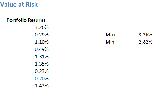
Step 1 – From the given time series (of portfolio returns) calculate the maximum and minimum return. To do this, we can use the ‘=Max()’ and ‘=Min()’ function on excel.
Step 2 – Estimate the number of data points. The number of data points is quite straight forward. We can use the ‘=count ()’ function for this.
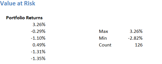
There are 126 data points, please do remember we are dealing with just last six months data for now. Ideally speaking, you should be running this exercise on at least 1 year of data. But as of now, the idea is just to push the concept across.
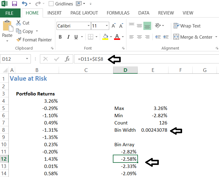
Step 3 – Bin width
We now have to create ‘bin array’ under which we can place the frequency of returns. The frequency of returns helps up understand the number of occurrence of a particular return. In simple terms, it helps us answer ‘how many times a return of say 0.5% has occurred over the last 126 day?’. To do this, we first calculate the bin width as follows –
Bin width = (Difference between max and min return) / 25
I’ve selected 25 based on the number of observations we have.
= (3.26% – (-2.82%))/25
=0.002431
Step 4 – Build the bin array
This is quite simple – we start form the lowest return and increment this with the bin width. For example, lowest return is -2.82, so the next cell would contain
= -2.82 + 0.002431
= – 2.58
We keep incrementing this until we hit the maximum return of 3.26%. Here is how the table looks at this stage –
And here is the full list –
We now have to calculate the frequency of these return occurring within the bin array. Let me just present the data first and then explain what is going on –
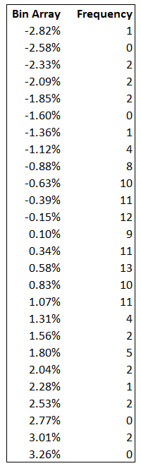
I’ve used the ‘=frequency ()’, function on excel to calculate the frequency. The first row, suggests that out of the 126 return observation, there was only 1 observation where the return was -2.82%. There were 0 observations between -2.82% and 2.58%. Similarly, there were 13 observations 0.34% and 0.58%. So on and so forth.
To calculate the frequency, we simply have to select all the cells next to Bin array, without deselecting, type =frequency in the formula bar and give the necessary inputs. Here is the image of how this part appears –
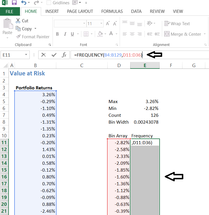
Do remember to hit ‘Ctrl + shift + enter’ simultaneously and not just enter. Upon doing this, you will generate the frequency of the returns.
Step 5 – Plot the distribution
This is fairly simple. We have the bin array which is where all our returns lie and next to that we have the frequency, which is the number of times a certain return has occurred. We just need to plot the graph of the frequency, and we get the frequency distribution. Our job now is to visually estimate if the distribution looks like a bell curve (normal distribution) or not.
To plot the distribution, I simply have to select the all the frequency data and opt for a bar chart. Here is how it looks –
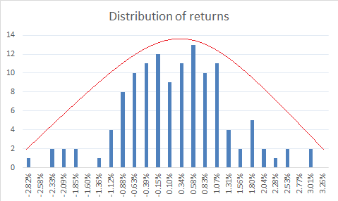
Clearly what we see above is a bell-shaped curve, hence it is quite reasonable to assume that the portfolio returns are normally distributed.
10.5 – Value at Risk
Now that we have established that the returns are normally distributed, we proceed to calculate the Value at Risk. From here on, the process is quite straightforward. To do this, we have to reorganize the portfolio returns from the ascending to descending order.
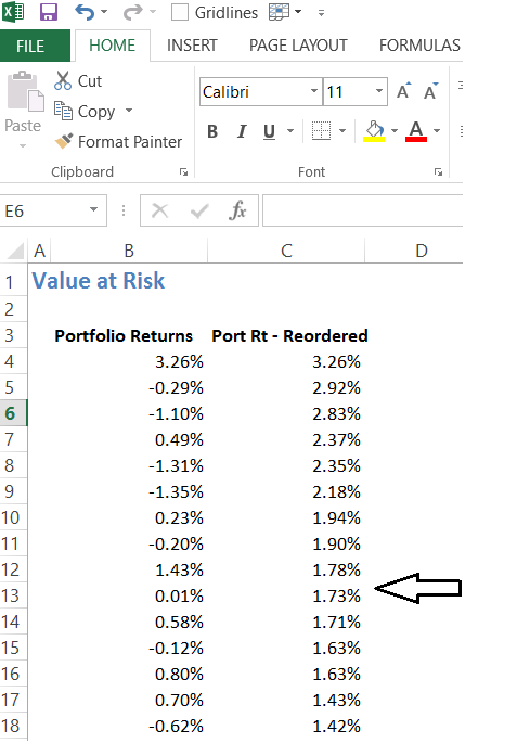
I’ve used excels sort function to do this. At this stage, I will go ahead and calculate Portfolio VaR and Portfolio CVaR. I will shortly explain, the logic behind this calculation.
Portfolio VaR – is defined as the least value within 95% of the observation. We have 126 observation, so 95% of this is 120 observations. Portfolio VaR is essential, the least most value within the 120 observations. This works out to be -1.48%.
I take the average of the remaining 5% of the observation, i.e the average of the last 6 observation, and that is the Cumulative VaR of CVaR.
The CVaR works out to -2.39%.
You may have many questions at this stage, let me list them down here along with the answers –
- Why did we plot the frequency distribution of the portfolio?
- To establish the fact that the portfolio returns are normally distributed
- Why should we check for normal distribution?
- If the data we are studying is normally distributed, then we can characteristics of normal distribution is applicable to the data set
- What are the characteristics of normally distributed data?
- There are quite a few, but you should specifically know that 68% of the data lies within 1 SD, 95% of the data within 2nd, and 99.7% of the data lies within the 3rd I’d suggest you read this chapter to know more about the normal distribution.
- Why did we sort the data?
- We have established that the data set is normally distributed. Do remember, we are only interested in the worst case scenario. Given this, when we sort it from highest to lowest, we are essentially in a position to look at the returns in a more systematic way.
- Why did bother to take only 95% observation?
- Remember, according to the normal distribution theory, 95% of the data lies within the 2nd standard deviation. This means on any random day, the return on the portfolio is likely to be any value within the 95% of the observations. Therefore, quite naturally the least most value within the 95% observation should represent the worst case loss or the Value at Risk.
- What does the VaR of -1.48% indicate?
- It tells that the worst case loss for the given portfolio is -1.49% and we can conclude this with a confidence of 95%
- Can’t the loss not exceed -1.48%?
- Yes, it certainly can and this is where CVaR comes into play. In the case of an extreme event, there is a 5% chance that the portfolio could experience a loss of -2.39%.
- Can’t the loss exceed beyond -2.89%?
- Yes, it can but the probability of this occurring is quite very low.
I hope the above discussion makes sense, do apply this on your equity portfolio and I’m sure you will gain a greater insight into how your portfolio is positioned.
We have discussed quite a few things with respect to the portfolio and the risk associated with it. We will now proceed to understand risk with respect to trading positions.
Download the Excel workbook used in this chapter.
Key takeaways from this chapter
- Events which have a very low probability of occurrence is called ‘Black Swan ’events
- When a black swan event occurs, a portfolio can experience higher levels of losses
- Value at Risk is one approach to estimate the worst case loss if a black swan event were to occur
- We can estimate the portfolio VaR by studying the distribution of the portfolio returns
- The average of the last 5% of the observation gives us the Value at Risk of the portfolio.
Hello Sir,
Could you please explain how did the number of observations come up to 25 because the count is 126. Apologies for the stupid question
Ah you are talking about the bin width? That is an arbitrary choice, no logic 🙂
Yes, So i can take the number of observations in for bin width 30 or 50 and and it wont matter?
Yes, you can.
Is it safe to assume that any given portfolio follows ND? If yes I can directly go ahead and calculate 2SD to find my VaR, right?
Most EQ instruments and EQ-related portfolios follow ND. Yes, you can.
HAPPY NEW YEAR KARTHIK. I HAVE A QUESTION
FROM WHERE DID YOU LEARNED ABOUT THIS RISK MANAGEMENT ?
Happy new year to you as well! Everything one learns is from the markets itself 🙂
Sir,
As you suggested that to follow the efficient frontier, I would need to re-check and re-validate. I feel this would require similar attention like hedging. Personally for me, it would become very challenging like the hedging.
In this respect, could you kindly suggest a more traditional way to place weights on each of the stocks out of total investment wealth, in case of people like me who would find it difficult to tally and maintain the ratios as per market fluctuations. I would be very happy to receive suggestion on this.
One of the easiest path to take is going equal weight, Anirban 🙂
Sir,
I have been learning through your modules from the beginning and personally to me, this 9th module is the best I found till the time. I have tried to slowing grasp understanding the market. However, I am still to make a good understanding on the macro trends/ economics that influences the market. Thus, I want to know that could you suggest an article/ book that will specially teach on this. Felt that mere reading NCERT or any good economics will not help much in this aspect. Require your kind advice here please.
Happy to note that, Anirban and I\’m glad you liked all the content here 🙂
I\’m not sure if I can recommend any simple macro economic books. In fact, I\’d like to know if you ever come across one 🙂
Sir,
What will be the look back period to consider data for calculation to arrive at deciding the weights we should consider of each of the stocks in our long horizon (20-25 years) portfolio?
You can start with 3 years data, but the most important thing to note is that you need to keep reevaluating this every year.
Sir,
You have shown calculation of portfolio variance through matrix multiplication and equity curve as well. Then can we go through any of the modes to calculate the same?
Yes, you can do that.
Sir,
To minimize risk, we have learnt to distribute through various sectors with different stock. Now, I am going through your chapter, \”Value at risk\” and thought to take suggestion for —— Should we equally look to make investments in foreign stocks too, to decrease the risk in other way? What will be your suggestion?
You can. Maybe via index funds.
Sir,
Can I follow this efficient frontier graph even for 25 years buy and hold strategy?
You will have to keep rechecking and validating it.
Sir,
In the efficient frontier graph, there is a min/max return corresponding to every risk taken. However, for the least risk, the graph is showing only the \”expected portfolio return\” data. Now, suppose, in a case, somebody wants to invest in such a way that the risk should be the minimum with highest return possible, then what should be his call?
Al portfolios on the efficient frontier curve are such portfolios only i.e max return for the given amount of risk.
Sir, what if the portfolio is NOT normally distributed,or its just like the portfolio will always be normally distributed and if not, what can we do to make a portfolio a normally distributed.
Stock returns are normally distributed whereas the stock prices are not. Hence the portfolio will be normally distributed.
SIR AFTER CONSTRUCTION OF PORTFOLIO . FROM THIS PORTFOLIO CAN WE GO FOR BETA HEDGEING WITH NIFTY SIR ?
Yes, provided you are confident of executing the strategy.
If we are dealing with 1 week return
Which data should consider. like, weekly data or yearly data
If weekly how many weeks need to take minimum?
For intraday how to consider data range ?
When you say dealing with 1-week data, what exactly do you intend to do? Calculate just the returns or use the weekly data for pattern analysis. Answers depend on what you intend to achieve.
> It tells that the worst case loss for the given portfolio is -1.49% and we can conclude this with a confidence of 95%
Is 1.49 a typo?
No, why do you think so?
Sir while calculating bin width why did you used 25. Any specific reason ? What number we will use ??
No specific reason for it. Its based on the number of data points. I use a thumb rule as 25 bins for every 500 data points.
Assuming a plot is normal needs justification. Visual justification is not enough. There are sound statistical tests for that. Typically financial data has \”fatter tails\” than a normal distribution and this can result in incorrect estimation of returns at the extremities.
Yes, you do have a point. Will try and add these things to the process as well.
Sir in bin width how the observation 25 is found?
it should be 126 know.
There is no fixed rule for this. Its just based on your convenience. I could have taken 50 bins also.
So there is no benefit in creating a portfolio ourself?
There is, provided you know what stocks you are picking and the thesis behind it.
Hi again,
I had another question.
I understand that someone who is looking to get a job within this field would be interested in learning about these concepts. And maybe someone who is curious would also find this information very interesting and valuable. But majority of the investors don\’t have the patience or the time to go through 10s of books to educate themselves in this field just to create a portfolio. Infact most don\’t even check the basic fundamentals of a company let alone optimising the portfolio. So why don\’t people just invest in mutual funds. After all isn\’t it true that fund managers do all of this work to come up with a good portfolio that has fundamentally strong companies and optimised asset allocation and all of this for a minimal fees. Then why don\’t people just prefer mutual funds over direct exposure. Or is there a benefit to creating a well optimised portfolio ourself apart from no asset management fees.
Absolutely, that\’s why mutual funds are a great vehicle for investment. If you don\’t have the patience or time, invest in a fund and you can still achieve all your financial goals 🙂
Hi,
I have been reading this module lately and I have a request to make, i don\’t know where this belongs so I am just posting it here. I want to learn more in depth about mathematics involved in portfolio management similar to what has been discussed in this module. Can you suggest some good books or maybe other resources relating to this topic.
Regards
Jeevesh, you can check this book – \’Qunatitiatve Portfolio Technique\’. I forget the author\’s name, but I think its a good book to get your started.
Hi Kartik,
Does this risk matter if one is not leveraged and not dependent on their portfolio for living costs? Assuming that the underlying companies are stable businesses with little to no chance of insolvency.
Thanks,
This is good to know risk as you\’ll get a fair sense of how much you will lose in case of an extreme movement in a day.
Hello Karthik Sir,
Thank you for this wonderful chapter.
I have one doubt. What in case the distribution is not normal? How can we calculate the VaR in that case.
Regards
Stock prices may not be normal, but stock returns are Sangeet.
Hey Karthik, why have you taken the number of observations as 25 for 126 data points? Is there any methodical way we need to approach this? For instance, if there are 500 data points instead of 126, should the number 25 change to something else and if so, how do we determine it?
It\’s just an approximation. No hard and fast rule. Could have been 15 also. For 500, I\’d probably take 50 max.
When drawing the normal distribution, why can\’t we just plot the individual returns and the frequency of the same, why do we need to move with the bin approach
How else would you plot this?
Respected sir,
Firstly thank you for these modules, the content is amazing as always. And as always I have a doubt too! Apparently, I was able to follow you through till the end except when you briefly mentioned this- Portfolio VaR is essential, the least most value within the 120 observations. This works out to be -1.48%. How did you get -1.48%? Utterly befuddled!
Thanks in advance:)
Aarti, that would be the least value in the top 120 data points, remember we need to look at 95% of values from the entire data set. Do download the excel, that should clear up the doubt.
I Really Appreciate Your Knowledge. thanks for this post..👍👍👍
Happy reading!
Hi ,
I was trying to recreate the excel file to accomodate a years worth of data. So , i tried having the same set of data for 6 months and tried to extrapolate and somehow the numbers did not match.
I looked through each and every line and then found out that the \”RT Average \” column is taken from the cell C 55 and not C5 for everything.
Is this done intentionally ?
That is to take the worst 5 returns and its average I supposed. I guess I have explained the same in the chapter.
is value at risk and lower circuit are similar or they have some difference
They are completely different 🙂
Hey there, Karthik!
What would be the denominator number (instead of 25) for calculating bin width incase of last 1 year data?
For 1 year, maybe 12 or 15 should do?
Pl allow buy risk penny stock
sir if -1.48% is daily var, then how can we find annual percentage as VAR?
Also if observations are not normally distributed then, what should we do?
please help out..
thank you..
Think of the VaR as SD and you can annualise it the same way, but doing that would be futile as VaR is expected to give us the daily risk factor. If you are dealing with stock returns, then they are normally distributed, stock prices may not.
sir as per normal distribution theory, we should have taken 95% observations from center ie: leaving 3 observations from top and 3 from bottom. why did we not do that ?
We did that and sorted the values in order, right?
sir the number that we got as VAR ie: 1.48%, is this value for each day or after a month or year? Please help me out..
That\’s a daily value.
Thank you
Welcome!
Hi,
Two questions.
– how good are these return and risk principles in real life? If I take daily return based on last one year in bull market, and if the following year is not a bulk, then it will not work right ? Or do we have to take like last 10 years of data ? Are these used in real life ?
– As a retail trader how do I put these to use in real life. Say a budget of 1.5-2 lakh to invest? Should one go by fundamental, technical or portfolio return theory.
– is there any tool that l, if fed with 5 stock names comes up with these numbers of max return and risk..?
Kindly let me know. Thanks.
Ankit, I\’m not sure if there are any portfolio analytics software which gives you these metrics. VaR as a concept generally tends to help large portfolios, but that said there is no rule which says you should not apply these concepts to smaller portfolios. I would suggest you do the drill and see where your portfolio stands in terms of risk and reward.
yes very much Karthik.Its your writing at varsity that has helped me to take a sensible and calculated approach towards trading which earlier i was having more of a gamblers approach.
Thanks a lot for that 🙂
Happy to note that, Shambu and I\’m so glad that you are enjoying the content here on Varsity!
the kind of build up that you do to every topic is absolutely mesmerizing and makes reading even interesting.
if world faces a black monday again and trading would stop forever,you need not worry still.
you would still take up carrier in writing and end up being a very good writer in deed,giving one best seller after another 😀
Hahah, that would be too much, Shambu. But I do hope you are enjoying reading on Varsity 🙂
Sir I think that this particular module is the most important contribution in your part to the common people. Thanks to your guiding hands, in the last few months I\’ve taken a major part of my money that was in FD and I\’ve invested them in \’Investment grade\’ stocks. However I\’m just getting started with portfolio optimization and management. Sir my question is, I\’ve read some books on finance and there seems to by contradictory views among the finance veteran s themselves. For instance I\’ve heard people say its not possible for an investor to time the market. But I recently read an entire book by Howard Marks on how to do the same. Even you said that some of the techniques in this module are keep a secret by high priests of finance. I guess my question is, how do you learn these things that people on top of the chain use? Your thoughts on this would help me a great deal. Thanks for varsity. Keep rocking sir.
The only difference here is the experience. By experience I mean the time spent in the market, observing markets, market cycles, the behavior of market participants etc. These things cannot be taught, you will have to tune your mind to this. Good luck, Sundeep.
Hi Karthik
The above calculations are valid only if the distribution is normal. What if the returns are not normally distributed ? Apologies If I am missing something here.
The stock price returns are assumed to be normal. Anyway, if the return distribution are not normal, then I guess you notch up your SD values.
Now big fund houses manage there black swan day by hedging strategies. At 1987 these kind of strategies were there to handle crash ? What are the hedging strategies we should know ?
Whatever I\’ve known, I\’ve put it up here 🙂
Sure karthik. Will wait for your response Thnx
Sure, thanks so much.
Hi Karthik,
At the outset I would like to mention that you are just Awesome!.I am doing FRM and reading your articles help me a lot You nailed it when comes to explaining the most complicated things into most lucid manner. I am a big fan of you sir!
Well my question is bit off track but I\’m not getting any clue or answers which can help me out. Can you please help me to understand how we can compute RNIVs (Risks not captured in VaR) May be an excel sheet or some examples with number crunching will be of help. Thnx Chetan
Chetan, thanks so much for the kind words 🙂
Frankly, RNIV is new to me, I need to figure this out myself. Hopefully soon 🙂
Hi Karthik,
Can VaR be used for day trading taking NSE equity VaR reports that are published daily, if possible can you elaborate.
Hmm, I\’m not sure if it\’s of any help for active trading. You can get a sense of how risky your portfolio is.
Hi Karthik,
Thanks for your response, can you point to links to study this further.
I am new to stock market. So, should the VAR be maximum or minimum….?
Does not matter if you are new or old, VaR should be manageable (max or min does not matter as long you can manage the risk).
\”I’ve selected 25 based on the number of observations we have.\”….I didn\’t get you here sir.Why 25 became the\” number of observations\”???
The number of observation is the number of data points. So based on that, I\’ve opted for 25 as the number of bins.
Hi Karthik
NSE website has the data of VaR for each stock listed and also we get the VaR report at the end of the day (https://www.nseindia.com/products/content/equities/equities/homepage_eq.htm ). So can the VaR of each stock multiplied by its weightage in our portfolio, summing up would give the similar result of the worst-case scenario?
Hmmm, this can be a quick and dirty method. Works alright if you ask me.
There is tension rising between India and China over Doklam issue. China is constantly threatening us for the war. There is also tension rising up between the US and North Korea and the former is losing up its patience. Can this be the next Black Swan moment?
Should I consider selling all of my investment before it\’s too late?
I cannot advise you on what you need to do with your investments. But yeah, it\’s always a good thing to prepare for the worst and have a plan b.
I\’m little confused right now
Confused about? I\’ll be glad to help.
hi
i am looking for more clarity on this….suppose set of companies are consistently making profit from operating activities and at the same time global-domestic markets are bearish/bleeding…in this situation do the profit making companies share prices react to the market direction or it will go on its own….what extent profit making companies/institutions will hit by 2008 like crisis happened again…if i am right soon or later it will happen…thank you
From my experience, I\’ve noticed that macro economic conditions affect all companies across industries. Eventually, companies with great moats and corporate governance will eventually triumph. Their stock price, along with other companies also fall, but the difference is that they are the ones which will bounce back first after such a slump.
thank you…
Welcome!
Hi Karthik,
Thanks. Will you be covering Sharpe ratio, risk aversion coefficient, utility score etc in this module?
Waiting for next chapter.
Thanks & regards ?
Will be talking about position sizing next. Maybe cover the topics you mentioned as a supplementary note.
Hi Karthik,
Can you please kindly explain how this frequency() function works.
In excel sheet, the frequency for 3.26% shows as \”zero\”. It isn\’t clear to me.
Thanks & Regards ?
Santosh
You need to ensure that all the cells are selected. Once done, goto the formula editor, open the frequency function and feed in the data. Close the brackets and press control shift enter. All this without deselecting the cells.
Desperately waiting for the trading strategies module . I will start trading only after that. By delaying it you are costing Zerodha millions of rupees of brokerage Karthik haha.
Karan, sure, I\’ll try my best to finish this module and get started on Trading Strategies.
when u gonna start nodule 10 of trading strategies ??? cant wait >.<
Waiting for this module to get over!
Respected Sir,
Nice chapter to understand VaR concept along with its importance. In addition to the queries posted above, I want to know why you have considered 3.26% (highest return) as the starting point for 95% confidence span. As per the Normal Distribution pattern, the 95% confidence span is around the central (average) point, i.e. Avg-2SD and Avg+2SD. This means that about 2.5% (3-4 observations) from highest & 2.5% (3-4 observations) from lowest should not be considered.
In short, the 95% confidence span must start somewhere from 2.83% (not 3.26%), & hence, VaR must be -2.33% (not-1.48%). Please clarify.
Thanks & Regards
James
Good observation, James. When dealing with VaR, we are not considering the symmetry of the data, we are interested in covering 95% of the data.
Hi Karthik,
Thanks for the yet another great insightful chapter on topic of VaR, CVaR.
Just few clarification needed: for calculating bin width you took 25 saying that it is based on observation which is 126. How did u arrive at 25, not quite clear to me. Is there any ratio/proportion for number of given data points. What if data points are more let\’s say 300, then what should be our number? 25, greater than 25 or less than 25? Kindly elobrate the same.
what I understood is that it is just assumed number only to check for NormalDistribution pattern. But it shud not be too big or too small. Am i correct?
Thanks & Regards ?
Hmm, there is no benchmark as such, or at least I\’m not aware of this. If you have something like 300 data points, then I\’d still take 25 bins….500 and above maybe 50. 2000+ maybe 75….but not really more than 75 I guess.
I learned something similar in statistics! That for a distribution to give valid probabilities or confidence limit , it should be based on at least a sample size of 30 ….why this 30..and even my teacher didn\’t know really ! But what I guess is that this number is actually established by real experiments of testing of various distributions in real life!
This must be based on some empirical observation. I\’m not sure about this, Madhhukar 🙂
This VaR is not so bad because last 6 months data is from bull market, right?
if we take data points from bear market then this value would be large.
so my question is still it does not reflect how my portfolio will behave in event of black Monday. (suppose Nifty drops suddenly by 10%)
True, last 6 months have been great for markets. Ideally, you should take at least last 1-year data point.