4.1 – A quick recap

Let us begin this chapter with a quick recap of our discussion so far.

We started this module with a discussion on the two kinds of risk a market participant is exposed to, when he or she purchases a stock – namely the systematic risk and the unsystematic risk. Having understood the basic difference between these two types of risk, we proceeded towards understanding risk from a portfolio perspective. In our discussion leading to portfolio risk or portfolio variance, we discussed two crucial concepts – variance and co variance. Variance is the deviation of a stock’s return with its own average returns. Co variance on the other hand is the variance of a stock’s return with respect to another stocks’ return. The discussion on variance and co variance was mainly with respect to a two stock portfolio; however we concluded that a typical equity portfolio contains multiple stocks. In order to estimate the variance co variance and the correlation of a multi stock portfolio, we need the help of matrix algebra.

So that’s where we are as of now.

In this chapter we will extent this discussion to estimate the ‘variance co variance’ of multiple stocks; this will introduce us to matrix multiplication and other concepts. However, the ‘variance covariance’ matrix alone does not convey much information. To make sense of this, we need to develop the correlation matrix. Once we are through with this part, we use the results of the correlation matrix to calculate the portfolio variance. Remember, our end goal is to estimate the portfolio variance. Portfolio variance tells us the amount of risk one is exposed to when he or she holds a set of stocks in the portfolio.

At this stage you should realize that we are focusing on risk from the entire portfolio perspective. While we are at it we will also discuss ‘asset allocation’ and how it impacts portfolio returns and risk. This will also include a quick take on the concept of ‘value at risk’.

Of course, we will also take a detailed look at risk from a trader’s perspective. How one can identify trading risk and ways to mitigate the same.

4.2 – Variance Covariance matrix

Before we proceed any further, I’ve been talking about ‘Variance Covariance matrix’. Just to clear up any confusion – is it ‘variance covariance matrix’ or is it a variance matrix and a covariance matrix?  Or is it just one matrix i.e the ‘Variance Covariance matrix’.

Well, is it just one matrix i.e the ‘Variance Covariance matrix’. Think about it, if there are 5 stocks, then this matrix should convey information on the variance of a stock and it should also convey the covariance of between stock 1 and the other 4 stock. Soon we will take up an example and I guess you will have a lot more clarity on this.

Please do note – it is advisable for you to know some basis on matrix operations. If not, here is a great video from Khan Academy which introduces matrix multiplication –

Anyway, continuing from the previous chapter, let us now try and calculate the Variance Covariance matrix followed by the correlation matrix for a portfolio with multiple stocks. A well diversified (high conviction) portfolio typically consists of about 10-15 stocks. I’d have loved to take up a portfolio of this size to demonstrate the calculation of the variance covariance matrix, but then, it would be a very cumbersome affair on excel and there is a good a newbie could get intimidated with the sheer size of the matrix, hence for this reason, I just decided to have a 5 stock portfolio.

The following 5 stocks constitutes my portfolio –

1. Cipla
2. Idea
3. Wonderla
4. PVR
5. Alkem

The size of the variance covariance matrix for a 5 stock portfolio will be 5 x 5. In general, if there are ‘k’ stocks in the portfolio, then the size of the variance covariance matrix will be k x k (read this as k by k).

The formula to create a variance covariance matrix is as follows –

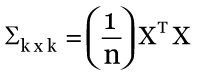
Where,

k = number of stocks in the portfolio

n = number of observations

X = this is the n x k excess return matrix. We will understand this better shortly

X^T  = transpose matrix of X

Here is a quick explanation of what is going on in that formula. You may understand this better when we deal with its implementation.

In simple terms, we first calculate the n x k excess return matrix; multiply this matrix by its own transpose matrix. This is a matrix multiplication and the resulting matrix will be a k x k matrix. We then divide each element of this k x k matrix by n, where n denotes the number of observations. The resulting matrix after this division is a k x k variance covariance matrix.

Generating the k x k variance covariance matrix is one step away from our final objective i.e getting the correlation matrix.

So, let us apply this formula and generate the variance covariance matrix for the 5 stocks listed above. I’m using MS excel for this. I have downloaded the daily closing prices for the 5 stocks for the last 6 months.

Step 1 – Calculated the daily returns. I guess you are quite familiar with this by now. I’m not going to explain how to calculate the daily returns. Here is the excel snapshot.

 

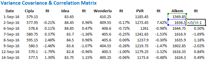
As you can see, I’ve lined up the stock’s closing price and next to it I have calculated the daily returns. I have indicated the formula to calculate the daily return.

Step 2 – Calculate the average daily returns for each stock. You can do this by using the ‘average’ function in excel.

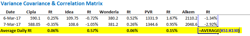
Step 3 – Set up the excess return matrix.

Excess return matrix is defined as the difference between stock’s daily return over its average return. If you recall, we did this in the previous chapter while discussing covariance between two stocks.

I’ve set up the excess return matrix in the following way –

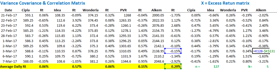
Do note, the resulting matrix is of n x k size, where n represents the number of observations (127 in this case) and k denotes the number of stocks (5 stocks). So in our example the matrix size is 127 x 5. We have denoted this matrix as X.

Step 4 – Generate the X^T X matrix operation to create a k x k matrix

This may sound fancy, but it is not.

X^T is a new matrix, formed by interchanging the rows and columns of the original matrix X. When you interchange the rows and columns of a matrix to form a new one, then it is referred to as a transpose matrix of X and denoted as X^T. Our objective now is to multiply the original matrix with its transpose. This is denoted as X^T X.

Note, the resulting matrix from this operation will result in a k x k matrix, where k denotes the number of stocks in the portfolio. In our case this will be 5 x 5.

We can do this in one shot in excel. I will use the following function steps to create the k x k matrix –

List down the stocks in rows and columns –

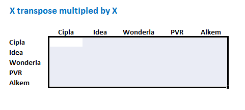
Apply the function = ‘MMULT ((transpose X), X). Remember X is the excess return matrix.

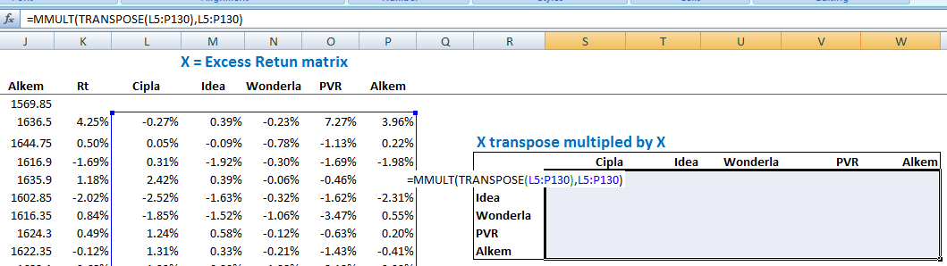
Do note, while applying this formula, you need to ensure that you highlight the k x k matrix. Once you finish typing the formula, do note – you cannot hit ‘enter’ directly. You will hit ctrl+shift+enter. In fact, for all array functions in excel, use ctrl+shift+enter.

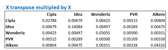
So once you hit ctrl+shift+enter, excel will present you with a beautiful k x k matrix, which in this case looks like this –

Step 5 – This is the last step in creating the variance covariance matrix. We now have to divide each element of the X^T X matrix by the total number of observations i.e n. For your clarity, let me post the formula for the variance covariance matrix again –

Again, we start by creating the layout for k x k matrix –

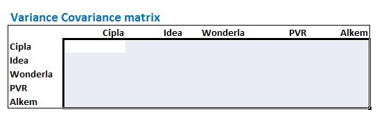
Once the layout is set, without deselecting the cells, select the entire X^T X matrix and divide it by n i.e 127. Do note, this is still an array function; hence you need to hit ctrl+shift+enter and not just enter.

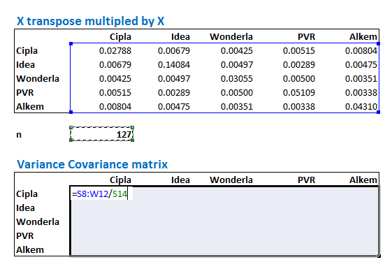
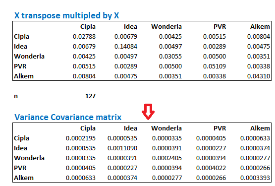
Once you hit control shift enter, you will get the ‘Variance – Covariance’ matrix. Do note, the numbers in the matrix will be very small, do not worry about this. Here is the variance co variance matrix –

 

Let us spend some time to understand the ‘Variance – Covariance’ matrix better. Suppose I want to know the covariance between any two stocks, lets say Wonderla and PVR, then I simply have to look for Wonderla on the left hand side and in the same row, look for the value which coincides with PVR. This would be the covariance between the two stocks. I’ve highlighted the same in yellow –

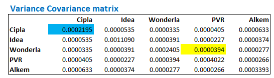
So the matrix suggests that the covariance between Wonderla and PVR is 0.000034. Do note, this is the same as the covariance between PVR and Wonderla.

Further, notice the number highlighted in blue. This value corresponds to Cipla and Cipla. What do you this represents? This represents the covariance between Cipla and Cipla, and if you realize, covariance of a stock with itself, is nothing but variance!

This is exactly why this matrix is called ‘Variance – Covariance Matrix’, cause it gives us both the values.

Now, here is the bitter pill – the variance and covariance matrix on its own is quite useless. These are extremely small numbers and it is hard to derive any meaning out of it. What we really need is the ‘Correlation Matrix’.

In the next chapter, let us deal with generating the correlation matrix, and also work towards estimating the portfolio variance, which is our end objective. However, before we close this chapter, here are few tasks for you –

1. Download the last 1 year data for 5 or more stocks.
2. Calculate the Variance – Covariance matrix for the same
3. For a given stock, identify the variance value. Apply the = ‘Var()’ function on excel on the returns of the same stock and evaluate if both are matching.

You can download the excel sheet used in this chapter.

---

Key Takeaways from this chapter

1. X is defined as an excess return matrix
2. Excess return matrix is simply the time series difference daily return versus the average daily return
3. X^T is defined as the transpose of X
4. Variable n is defined as the number of observations in the data set. For example if you have 6 months data, n is 127, for 1 year data n would be 252
5. Excess return matrix is of the size n x k, where k is the number of stocks
6. When you divide the matrix product of X^T X by n, we get the variance covariance matrix
7. The variance covariance matrix is of the size k x k
8. The covariance of stock 1 with itself is the variance of stock 1
9. The variance covariance matrix will lead us to the correlation matrix.