5.1 – Revisiting the Normal Distribution

If you have been a regular reader on Varsity, then chances are you’d have come across the discussion on Normal Distribution in the Options Module. If you’re not, then I’d strongly suggest you read up this chapter on Normal distribution.

This is a very important topic, I’d suggest you spend some time reading about it before you proceed. We will use the concept of Normal Distribution in both the techniques of Pair Trading, i.e the Mark Whistler’s Pair Trading technique, and the other technique we will discuss later on in this module. Given the central role it plays, you should spend time reading about it.

I’m reproducing the central theme around Normal distribution, this should serve as a quick refresher for people who are familiar with Normal Distribution, but for those who are not, I hope this does not demotivate you from reading the chapter on Normal distribution –

The general theory around the normal distribution which you should know –

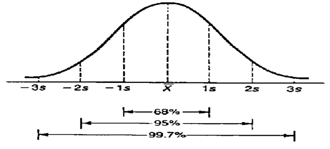
• Within the 1^st standard deviation, one can observe 68% of the data
• Within the 2^nd standard deviation, one can observe 95% of the data
• Within the 3^rd standard deviation, one can observe 99.7% of the data

The following image should help you visualize the above –

Of course, there are other forms in which the data gets distributed – distribution such as uniform, binomial, exponential distribution etc. This is just for your information.

5.2 – Descriptive Statistics

In the previous chapter, we discussed three basic statistical metrics namely the Mean, Median, and Mode. We will now calculate these metrics on the pair data i.e the differential, spread, and ratio which we computed in the previous chapter. We will do these calculations using the excel functions.

Please note, I’m continuing on the excel that we were working on in the previous chapter, needless to say, you can download the updated excel from the link provided towards the end of the chapter.

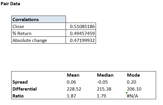
The sheet is set up as below –

The Excel functions are as follows –

1. Mean – ‘=average()’
2. Median – ‘=median()’
3. Mode – ‘=mode.mult()’

And the numbers are as below –

As you may notice, the correlation numbers were calculated in the previous chapter.

We now have the data setup. We need to add one key variable here and that would be the standard deviation. Again, standard deviation as a concept has been explained in Varsity earlier. I’d suggest you read this chapter to understand Standard Deviation better. Here is the summary though –

Standard Deviation simply generalizes and represents the deviation from the average. Here is the textbook definition of SD “In statistics, the standard deviation (SD, also represented by the Greek letter sigma, σ) is a measure that is used to quantify the amount of variation or dispersion of a set of data values”.

So in a sense, Standard Deviation gives us a sense of variability of the data or in other words, help us understand how widely the data set is spread out. Let me try and put this in the context of the Pair data we are dealing with.

The differential data which we computed a while ago is something like this –

Together there are 496 differential data points and earlier in this chapter, we have even calculated the average value across these data points i.e 228.52.

Now, what if I were to ask you to help me understand the variability of these data points from its average value? Or a better question to ask – why would I need to know the variability of the data points from its average value?

Well, if we don’t know the variability of the data, then there is no way we can make an intelligent assessment of the behavior of the data set. For example, when the 498^th data is generated, we will know if this value is around the mean or within the range it varies.

This, in fact, forms the crux of pair trading.

Standard Deviation helps us measure this variation.

While I personally think standard deviation is good enough, there are traders who would also like to calculate another variable called the ‘Absolute Deviation’. Both standard deviation and absolute deviation help us understand the variability of the data. But they differ in terms of the way do they data is treated.

I was looking at the explanation to help you understand the difference between standard deviation and absolute deviation, and I found the following on Investopedia, which I think is quite nice. I’m taking the liberty of reproducing the content here –

“While there are many different ways to measure variability within a set of data, two of the most popular are standard deviation and average deviation. Though very similar, the calculation and interpretation of these two differ in some key ways. Determining range and volatility is especially important in the finance industry, so professionals in areas such as accounting, investing and economics should be very familiar with both concepts.

Standard deviation is the most common measure of variability and is frequently used to determine the volatility of stock markets or other investments. To calculate the standard deviation, you must first determine the variance. This is done by subtracting the mean from each data point and then squaring, summing and averaging the differences. Variance in itself is an excellent measure of variability and range, as a larger variance reflects a greater spread in the underlying data. The standard deviation is simply the square root of the variance. Squaring the differences between each point and the mean avoids the issue of negative differences for values below the mean, but it means the variance is no longer in the same unit of measure as the original data. Taking the root of the variance means the standard deviation returns to the original unit of measure and is easier to interpret and utilize in further calculations.

The average deviation, also called the mean absolute deviation, is another measure of variability. However, average deviation utilizes absolute values instead of squares to circumvent the issue of negative differences between data and the mean. To calculate the average deviation, simply subtract the mean from each value, then sum and average the absolute values of the differences. The mean absolute value is used less frequently because the use of absolute values makes further calculations more complicated and unwieldy than using the simple standard deviation.”

We will go ahead and compute both “Standard Deviation”, and “Absolute Deviation” for all the three pair data variables.

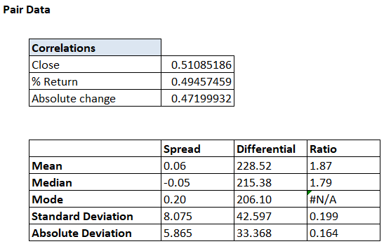
By the way, I’m interchanging the Y-axis to Mean, Median, and Mode. The X-axis to Differential, Ratio, and Spread. Given this, the snapshots posted above will be slightly different from the one posted below, hope you won’t mind my clumsy data handling skills J

The excel function to calculate these variables are –

Standard Deviation – ‘=Stdev.p()’

Absolute Deviation – ‘=avedev()’

The Mean, Median, Mode, Standard Deviation, and Absolute Deviation is also known as the basic descriptive statistics.

5.3 – The Standard deviation table

The standard deviation as you know helps us get a sense of the variation in the data. We will now take this a step further and try and quantify the variation. Why do we need to do this, you may ask? Well, this will help us understand the extent of the variation from the mean value. For example, the 498^th differential data could be 275, we will exactly know if 275 is way above the mean or way too below the mean.

With this information, we can choose to either buy the pair or short the pair. Of course, we will get into these details later on. For now, let us focus on quantifying the extent of the variation. In order to quantify the data point, we need to build something called as a standard deviation table.

The structure of the table is as below –

As you may have guessed, we are now going to calculate the values of 1, 2, and 3 standard deviations above the mean and below the mean, across spread, differential, and the ratio.

For example, let us just focus on the Spread data for now. The mean of the spread is 0.06. We also know the standard deviation (SD) is 8.075.

Therefore, the 1st SD above the mean would be –

0.064 + 8.075 = 8.139

2^nd SD –

0.064 + (2*8.075) = 16.123

3^rd SD –

0.064 + (3*8.075) = 24.288

These are all values above the mean. We can do the same to identify the values below the mean –

-1 SD –

0.064 – 8.075 = -8.011

-2 SD –

0.064 – (2*8.075) = -16.086

-3 SD –

0.064 – (3*8.075) = -24.160

I’ve done the same math across Differential and Ratio. Here is how the table looks –

So if the 498^th differential data read 315, then we can quickly understand that the value is around the +2 standard deviation and with 95% confidence you could conclude that there is only 5% chance for the next set of data points to go higher than 315.

Anyway, at this stage, we have almost all the data that we need to make the assessment of the pair and probably identify if there is an opportunity to trade. In the next chapter, we will go ahead and do this. In fact, I’ll start the next chapter with a quick recap of everything we have discussed so far, this is just to ensure we are all on the same page.

You can download the excel sheet used in this chapter here.

Signing of this chapter by wishing you all a very happy Xmas and a happy new year! Hope 2018 brings in wisdom, wealth, and peace your way.

---

Key takeaways from this chapter

1. Normal distribution plays a pivotal role in pair trading
2. Within the 1^st standard deviation, one can observe 68% of the data
3. Within the 2^nd standard deviation, one can observe 95% of the data
4. Within the 3^rd standard deviation, one can observe 99.7% of the data
5. Standard deviation and absolute deviation measures the variability of the data
6. The standard deviation table gives us a sense of how the current data stands with respect to its expected variation
7. The cues to trade the pair either long or short comes from the standard deviation table.