7.1 – Spreads versus naked positions

Over the last five chapters we’ve discussed various multi leg bullish strategies. These strategies ranged to suit an assortment of market outlook – from an outrightly bullish market outlook to moderately bullish market outlook. Reading through the last 5 chapters you must have realised that most professional options traders prefer initiating a spread strategy versus taking on naked option positions. No doubt, spreads tend to shrink the overall profitability, but at the same time spreads give you a greater visibility on risk. Professional traders value ‘risk visibility’ more than the profits. In simple words, it’s a much better deal to take on smaller profits as long as you know what would be your maximum loss under worst case scenarios.

Another interesting aspect of spreads is that invariably there is some sort of financing involved, wherein the purchase of an option is funded by the sale of another option. In fact, financing is one of the key aspects that differentiate a spread versus a normal naked directional position. Over the next few chapters we will discuss strategies which you can deploy when your outlook ranges from moderately bearish to out rightly bearish. The composition of these strategies is similar to the bullish strategies that we discussed earlier in the module.

The first bearish strategy we will look into is the Bear Put Spread, which as you may have guessed is the equivalent of the Bull Call Spread.

7.2 – Strategy notes

Similar to the Bull Call Spread, the Bear Put Spread is quite easy to implement. One would implement a bear put spread when the market outlook is moderately bearish, i.e you expect the market to go down in the near term while at the same time you don’t expect it to go down much. If I were to quantify ‘moderately bearish’, a 4-5% correction would be apt. By invoking a bear put spread one would make a modest gain if the markets correct (go down) as expected but on the other hand if the markets were to go up, the trader will end up with a limited loss.

A conservative trader (read as risk averse trader) would implement Bear Put Spread strategy by simultaneously –

1. Buying an In the money Put option
2. Selling an Out of the Money Put option

There is no compulsion that the Bear Put Spread has to be created with an ITM and OTM option. The Bear Put spread can be created employing any two put options. The choice of strike depends on the aggressiveness of the trade. However do note that both the options should belong to the same expiry and same underlying. To understand the implementation better, let’s take up an example and see how the strategy behaves under different scenarios.

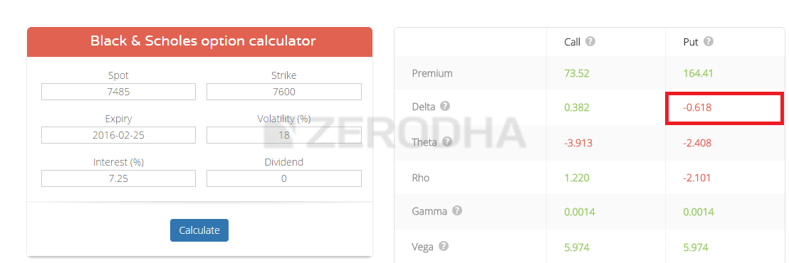
As of today Nifty is at 7485, this would make 7600 PE In the money and 7400 PE Out of the money. The ‘Bear Put Spread’ would require one to sell 7400 PE, the premium received from the sale would partially finance the purchase of the 7600 PE. The premium paid (PP) for the 7600 PE is Rs.165, and the premium received (PR) for the 7400 PE is Rs.73/-. The net debit for this transaction would be –

73 – 165

= -92

To understand how the payoff of the strategy works under different expiry circumstances, we need to consider different scenarios. Please do bear in mind the payoff is upon expiry, which means to say that the trader is expected to hold these positions till expiry.

Scenario 1 – Market expires at 7800 (above long put option i.e 7600)

This is a case where the market has gone up as opposed to the expectation that it would go down. At 7800 both the put option i.e 7600 and 7400 would not have any intrinsic value, hence they would expire worthless.

• The premium paid for 7600 PE i.e Rs.165 would go to 0, hence we retain nothing
• The premium received for 7400 PE i.e Rs.73 would be retained entirely
• Hence at 7800, we would lose Rs.165 on one hand but this would be partially offset by the premium received i.e Rs.73
• The overall loss would be -165 + 73 = -92

Do note the ‘-ve’ sign associated with 165 indicates that this is a money outflow from the account, and the ‘+ve’ sign associated with 73 indicates that the money is received into the account.

Also, the net loss of 92 is equivalent to the net debit of the strategy.

Scenario 2 – Market expired at 7600 (at long put option)

In this scenario we assume the market expires at 7600, where we have purchased a Put option. But then, at 7600 both 7600 and 7400 PE would expire worthless (similar to scenario 1) resulting in a loss of -92.

Scenario 3 – Market expires at 7508 (breakeven)

7508 is half way through 7600 and 7400, and as you may have guessed I’ve picked 7508 specifically to showcase that the strategy neither makes money nor loses any money at this specific point.

• The 7600 PE would have an intrinsic value equivalent to Max [7600 -7508, 0], which is 92.
• Since we have paid Rs.165 as premium for the 7600 PE, some of the premium paid would be recovered. That would be 165 – 92 = 73, which means to say the net loss on 7600 PE at this stage would be Rs.73 and not Rs.165
• The 7400 PE would expire worthless, hence we get to retain the entire premium of Rs.73
• So on hand we make 73 (7400 PE) and on the other we lose 73 (7600 PE) resulting in a no loss no profit situation

Hence, 7508 would be the breakeven point for this strategy.

Scenario 4 – Market expires at 7400 (at short put option)

This is an interesting level, do recall when we initiated the position the spot was at 7485, and now the market has gone down as expected. At this point both the options would have interesting outcomes.

• The 7600 PE would have an intrinsic value equivalent to Max [7600 -7400, 0], which is 200
• We have paid a premium of Rs.165, which would be recovered from the intrinsic value of Rs.200, hence after compensating for the premium paid one would retain Rs.35/-
• The 7400 PE would expire worthless, hence the entire premium of Rs.73 would be retained
• The net profit at this level would be 35+73 = 108

The net payoff from the strategy is in line with the overall expectation from the strategy i.e the trader gets to make a modest profit when the market goes down.

Scenario 5 – Market expires at 7200 (below the short put option)

This is again an interesting level as both the options would have an intrinsic value. Lets figure out how the numbers add up –

• The 7600 PE would have an intrinsic value equivalent to Max [7600 -7200, 0], which is 400
• We have paid a premium of Rs.165, which would be recovered from the intrinsic value of Rs.400, hence after compensating for the premium paid one would retain Rs.235/-
• The 7400 PE would have an intrinsic value equivalent to Max [7400 -7200, 0], which is 200
• We received a premium of Rs.73, however we will have to let go of the premium and bear a loss over and above 73. This would be 200 -73 = 127
• On one hand we make a profit of Rs.235 and on the other we lose 127, therefore the net payoff of the strategy would be 235 – 127 = 108.

Summarizing all the scenarios (I’ve put up the payoff values directly after considering the premiums)

Market Expiry	Long Put (7600)_IV	Short Put (7400)_IV	Net payoff
7800	0	0	-92
7600	0	0	-92
7508	92	0	0
7200	400	200	+108

Do note, the net payoff from the strategy is in line with the overall expectation from the strategy i.e the trader gets to make a modest profit when the market goes down while at the same time the losses are capped in case the market goes up.

Have a look at the table below –

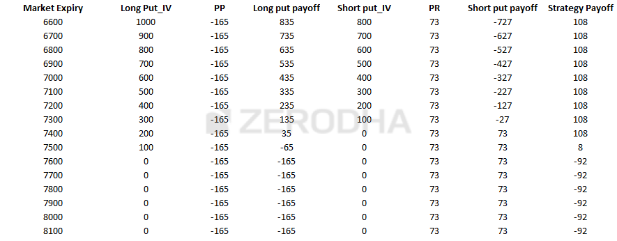
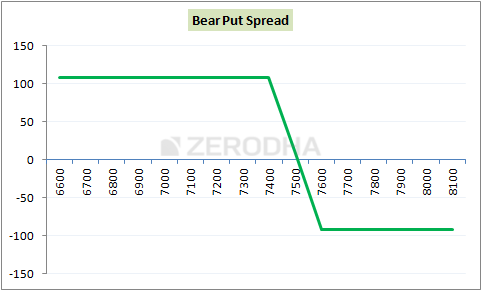
The table below shows the strategy payoff at different expiry levels. The losses are capped to 92 (when markets go up) and the profits are capped to 108 (when markets go down).

7.3 – Strategy critical levels

From the above discussed scenarios we can generalize a few things –

1. Strategy makes a loss if the spot moves above the breakeven point, and makes a profit below the breakeven point
2. Both the profits and loss are capped
3. Spread is difference between the two strike prices.
   1. In this example spread would be 7600 – 7400 = 200
4. Net Debit = Premium Paid – Premium Received
   1. 165 – 73 = 92
5. Breakeven = Higher strike – Net Debit
   1. 7600 – 92 = 7508
6. Max profit = Spread – Net Debit
   1. 200 – 92 = 108
7. Max Loss = Net Debit
   1. 92

You can note all these critical points in the strategy payoff diagram –

7.4 – Quick note on Delta

This is something I missed talking about in the earlier chapters, but its better late than never :-). Whenever you implement an options strategy always add up the deltas. I used the B&S calculator to calculate the deltas.

The delta of 7600 PE is -0.618

The delta of 7400 PE is – 0.342

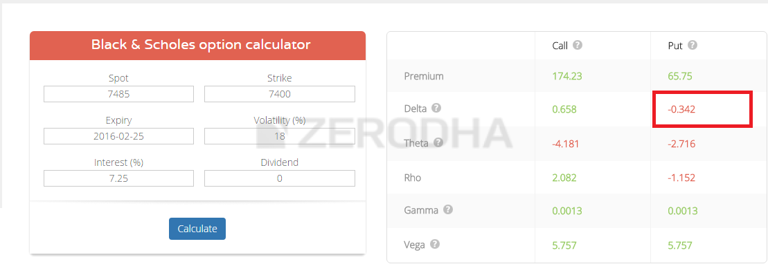
The negative sign indicates that the put option premium will go down if the markets go up, and premium gains value if the markets go down. But do note, we have written the 7400 PE, hence the Delta would be

-(-0.342)

+ 0.342

Now, since deltas are additive in nature we can add up the deltas to give the combined delta of the position. In this case it would be –

-0.618 + (+0.342)

= – 0.276

This means the strategy has an overall delta of 0.276 and the ‘–ve’ indicates that the premiums will go up if the markets go down. Similarly you can add up the deltas of other strategies we’ve discussed earlier – Bull Call Spread, Call Ratio Back spread etc and you will realize they all have a positive delta indicating that the strategy is bullish.

When you have more than 2 option legs it gets really difficult to estimate the overall bias of the strategy (whether the strategy is bullish or bearish), in such cases you can quickly add up the deltas to know the bias. Further, if in case the deltas add to zero, then it means that the strategy is not really biased to any direction. Such strategies are called ‘Delta Neutral’. We will eventually discuss these strategies at a later point in this module.

Also, you may be interested to know that while the delta neutral strategies are immune to market’s directional move, they react to changes in volatility and time, hence these are also sometime called “Volatility based strategies”.

7.5 – Strike selection and effect of volatility

The strike selection for a bear put spread is very similar to the strike selection methodology of a bull call spread. I hope you are familiar with the ‘1^st half of the series’ and ‘2^nd half of the series’ methodology. If not I’d suggest you to kindly read through section 2.3.

Have a look at the graph below –

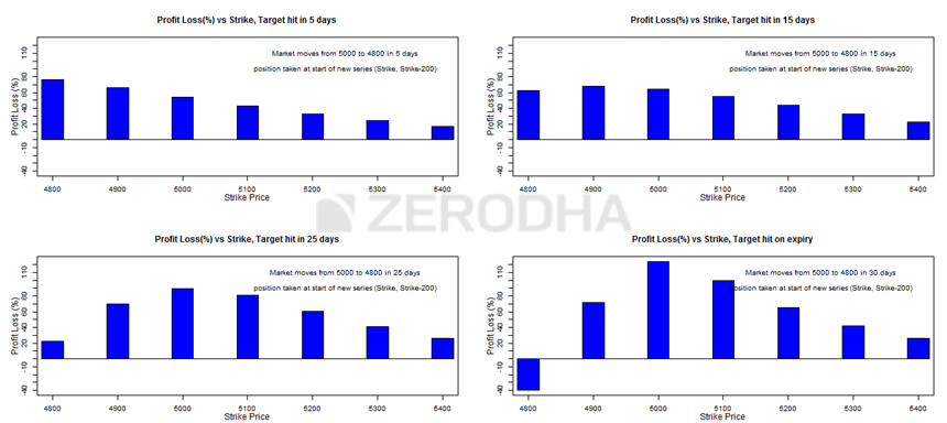
If we are in the first half of the series (ample time to expiry) and we expect the market to go down by about 4% from present levels, choose the following strikes to create the spread

Expect 4% move to happen within	Higher strike	Lower strike	Refer graph on
5 days	Far OTM	Far OTM	Top left
15 days	ATM	Slightly OTM	Top right
25 days	ATM	OTM	Bottom left
At expiry	ATM	OTM	Bottom right

Now assuming we are in the 2^nd half of the series, selecting the following strikes to create the spread would make sense –

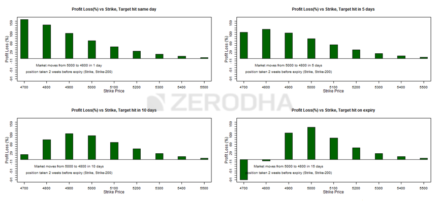
Expect 4% move to happen within	Higher strike	Lower strike	Refer graph on
Same day (even specific)	OTM	OTM	Top left
5 days	ITM/OTM	OTM	Top right
10 days	ITM/OTM	OTM	Bottom left
At expiry	ITM/OTM	OTM	Bottom right

I hope you will find the above two tables useful while selecting the strikes for the bear put spread.

We will now shift our focus on the effect of volatility on the bear put spread. Have a look at the following image –

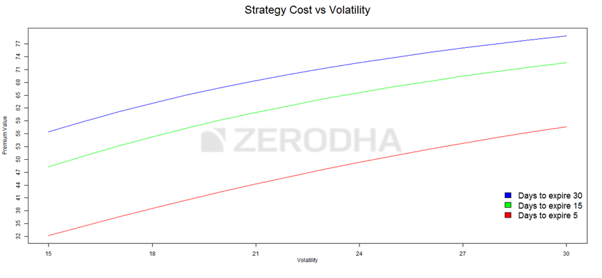
The graph above explains how the premium varies with respect to variation in volatility and time.

• The blue line suggests that the cost of the strategy does not vary much with the increase in volatility when there is ample time to expiry (30 days)
• The green line suggests that the cost of the strategy varies moderately with the increase in volatility when there is about 15 days to expiry
• The red line suggests that the cost of the strategy varies significantly with the increase in volatility when there is about 5 days to expiry

From these graphs it is clear that one should not really be worried about the changes in the volatility when there is ample time to expiry. However one should have a view on volatility between midway and expiry of the series. It is advisable to take the bear put spread only when the volatility is expected to increase, alternatively if you expect the volatility to decrease, its best to avoid the strategy.

---

Key takeaways from this chapter

1. Spread offers visibility on risk but at the same time shrinks the reward
2. When you create a spread, the proceeds from the sale of an option offsets the purchase of an option
3. Bear put spread is best invoked when you are moderately bearish on the markets
4. Both the profits and losses are capped
5. Classic bear put spread involves simultaneously purchasing ITM put options and selling OTM put options
6. Bear put spread usually results in a net debit
7. Net Debit = Premium Paid – Premium Received
8. Breakeven = Higher strike – Net Debit
9. Max profit = Spread – Net Debit
10. Max Loss = Net Debit
11. Select strikes based on the time to expiry
12. Implement the strategy only when you expect the volatility to increase (especially in the 2^nd half of the series)

 

Download Bear Put Spread Excel Sheet