16.1 – Market risk premium

In the previous chapter, we discussed that the equity holders expect a higher return than the debt holders. The higher return (rate) is what we will use to discount the free cash flow to the equity holders. But the question is, how much higher?

You can think about it this way: if the risk-free rate (Rf) is 7%, how much more would you like (over and above the risk-free rate) so that you feel encouraged to invest in equities? If you were to ask a bunch of investors and take an average of the expected return, you would arrive at the rate. However, most individual investors won’t have access to such a consensus. Hence we can probably apply an equation to get our answer.

Re = Risk free rate (Rf) + Risk premium

Where Re = Return expectation of equity holders.

The risk premium is the additional return over and above the risk-free return to encourage an investor to invest in equities. The risk premium is –

Risk premium = β*(Rm – Rf), where

Rf = Risk-free rate

Β = Beta of the stock

Rm = Market rate

Of course, we can rearrange the Re equation –

Re = Rf + β*(Rm – Rf)

By the way, this equation in finance is called ‘The Capital Asset Pricing model’ or CAPM.

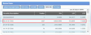
Let’s take an example and see how this works. The best proxy for the risk-free rate is the 10-year-old Govt bond yield. We can look it up on the CCIL portal –

I’ve highlighted the last traded yield of the 10-year Government bond maturing in 2032. The yield is 7.4586%. The yield indicates that if I were to invest in this bond and hold it for 10 years, I would earn a return of 7.4586% without any risk. Without any risk, because we don’t expect Govt of India to default on its debt obligations, default risk is almost non-existent.

Government defaulting on debt is a severe issue, so governments try their best not to default. Also, why are we considering 10 years and not any shorter-term bond? This is because we are interested in longer-term yields as we also forecast the free cash flow for the long term.

Next up is the Beta. Beta, as you may know, is the company’s stock price sensitivity with respect to the stock market. I’ve explained the concept of Beta and what it means in this chapter. I’d suggest you review it if you are not familiar with the idea of Beta as explained in section 11.5 of this chapter.

Rm is the market rate, and this is the market’s long-term average return. I’d suggest you keep this around 8% to 9%, maybe 10 or 12%, if you are bullish.

Please note that when we build the final model, all these rates can be changed to whatever you think makes sense. Let’s assume that the Beta of the company we are dealing with is riskier compared to market, and therefore we assign the Beta as 1.3.

By the way, you can easily calculate the Beta of any company in excel. Anyway, let us plug in these numbers and see how the return expectation of equity holders works –

= 7.4586% + (1.3) *( 8.5%-7.4586%)

= 8.81%

Of course, when we integrate this within our model, you are free to change the values to what you think makes sense. For example, if you feel the risk-free rate should be 8% instead of 7.45%, that’s fine, but whenever you make any change, make sure you have a reason for that change.

16.2 – Tax shield

In the last chapter, we learned that we could get the Free cash flow to the firm by adding non-cash expenses back to the Profit after taxes. The non-cash expenses included the following –

• • Depreciation
  • Amortization
  • Deferred taxes
  • Proceeds from the sale of assets
  • Interest expense

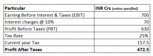
Adding the interest expense part is tricky, and we need to spend some time understanding how to add the interest. Let me take an arbitrary example to illustrate this, have a look at this –

As you can see, we have a fairly straightforward bottom line P&L of a company. The EBIT is 700 Crs, and the company pays 70Cr as interest charges at 10%. The PBT is 630 Crs, and at a 25% tax rate, the company pays a tax of 157.5Crs. The bottom line i.e. PAT = PAT – Taxes = 472.5 Crs.

Now, to calculate the Free cash flow to the firm, we start with PAT and add back non-cash expenses. We also add back the interest paid because the interest goes back to the debt holder of the company. If we were to do this –

PAT = 472.5

(Add) Interest = 70

= 542.5

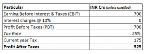
But there is a problem doing this. You see, when we pay interest, the tax outflow reduces. For instance, the tax here is 157.5 Crs while the interest paid is 70. Now, consider the interest as 0, this would make PBT 700, and at 25% tax, the tax outflow is 175.

So in a sense, interest shields us from a higher tax outflow. So interest that we add back should be factored in for tax shield. To do that –

Interest (with tax shield) = Interest *( 1 – tax)

= 70*(1-25%)
52.5

So when you add back interest to PAT to calculate the FCFF, we add 52.5 here and not 70. In this example –

PAT = 472.5

Interest = 52.5

525

Just to refresh, for FCFF calculation –

FCFF = PAT + Depreiciation + Amortization + Interest*(1-tax rate) + deferred taxes – working capital changes – investment in fixed assets (CAPEX).

We start the FCFF calculation with PAT, but instead, we can even begin with EBIT. If we were to start with EBIT, we need to add back the tax shield.

FCFF = EBIT *(1-tax rate)+ Depreiciation + Amortization + deferred taxes – working capital changes – investment in fixed assets (CAPEX).

Let’s plug in the above equation for the arbitrary example –

= 700*(1-25%)

= 525

Of course, for the sake of simplicity, I’ve ignored the non-cash expense, CAPEX, and working capital changes. But the point is that you can start your FCFF calculation with either PAT or EBIT; both will lead you to the same result.

You can extend the calculation to figure out the free cash flow to the equity holders by deducting the net debt from the free cash flow to the firm.

Free Cash flow to Equity = FCFF + [Debt – Principal repayment]

Where, [Debt – Principal repayment] = Net debt

Hence,

Free Cash flow to Equity = FCFF + Net debt

We will get back to this later when we implement the FCFF and FCFE within our model.

Key takeaways from this chapter

• • Equity investors expect a return over and above the risk-free rate and that is called the risk premium
  • The risk premium depends on the beta of the stock. Higher the beta, higher the premium
  • When the company pays interest, it gets a tax shield
  • When you add back in interest, you need to factor in the tax shield as well
  • You can start the calculation of Free cash flow either by PAT or by EBIT, both yield similar results