4.1 – Background
The Call Ratio Back Spread is an interesting options strategy. I call this interesting keeping in mind the simplicity of implementation and the kind of pay off it offers the trader. This should certainly have a spot in your strategy arsenal. The strategy is deployed when one is out rightly bullish on a stock (or index), unlike the bull call spread or bull put spread where one is moderately bullish.
At a broad level this is what you will experience when you implement the Call Ratio Back Spread-
- Unlimited profit if the market goes up
- Limited profit if market goes down
- A predefined loss if the market stay within a range
In simpler words you can get to make money as long as the market moves in either direction.

Usually, the Call Ratio Back Spread is deployed for a ‘net credit’, meaning money flows into your account as soon as you execute Call Ratio Back Spread. The ‘net credit’ is what you make if the market goes down, as opposed to your expectation (i.e market going up). On the other hand, if the market indeed goes up, then you stand to make an unlimited profit. I suppose this should also explain why the call ratio spread is better than buying a plain vanilla call option.
So let’s go ahead and figure out how this works.
4.2 – Strategy Notes
The Call Ratio Back Spread is a 3 leg option strategy as it involves buying two OTM call option and selling one ITM Call option. This is the classic 2:1 combo. In fact the call ratio back spread has to be executed in the 2:1 ratio meaning 2 options bought for every one option sold, or 4 options bought for every 2 option sold, so on and so forth.
Let take an example – assume Nifty Spot is at 7743 and you expect Nifty to hit 8100 by the end of expiry. This is clearly a bullish outlook on the market. To implement the Call Ratio Back Spread –
- Sell one lot of 7600 CE (ITM)
- Buy two lots of 7800 CE (OTM)
Make sure –
- The Call options belong to the same expiry
- Belongs to the same underlying
- The ratio is maintained
The trade set up looks like this –
- 7600 CE, one lot short, the premium received for this is Rs.201/-
- 7800 CE, two lots long, the premium paid is Rs.78/- per lot, so Rs.156/- for 2 lots
- Net Cash flow is = Premium Received – Premium Paid i.e 201 – 156 = 45 (Net Credit)
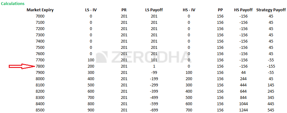
With these trades, the call ratio back spread is executed. Let us check what would happen to the overall cash flow of the strategies at different levels of expiry.
Do note we need to evaluate the strategy payoff at various levels of expiry as the strategy payoff is quite versatile.
Scenario 1 – Market expires at 7400 (below the lower strike price)
We know the intrinsic value of a call option (upon expiry) is –
Max [Spot – Strike, 0]
The 7600 would have an intrinsic value of
Max [7400 – 7600, 0]
= 0
Since we have sold this option, we get to retain the premium received i.e Rs.201
The intrinsic value of 7800 call option would also be zero; hence we lose the total premium paid i.e Rs.78 per lot or Rs.156 for two lots.
Net cash flow would Premium Received – Premium paid
= 201 – 156
= 45
Scenario 2 – Market expires at 7600 (at the lower strike price)
The intrinsic value of both the call options i.e 7600 and 7800 would be zero, hence both of them expire worthless.
We get to retain the premium received i.e Rs.201 towards the 7600 CE however we lose Rs.156 on the 7800 CE resulting in a net payoff of Rs.45.
Scenario 3 – Market expires at 7645 (at the lower strike price plus net credit)
You must be wondering why I picked the 7645 level, well this is to showcase the fact that the strategy break even is at this level.
The intrinsic value of 7600 CE would be –
Max [Spot – Strike, 0]
= [7645 – 7600, 0]
= 45
Since, we have sold this option for 201 the net pay off from the option would be
201 – 45
= 156
On the other hand we have bought two 7800 CE by paying a premium of 156. Clearly the 7800 CE would expire worthless hence, we lose the entire premium.
Net payoff would be –
156 – 156
= 0
So at 7645 the strategy neither makes money or loses any money for the trader, hence 7645 is treated as a breakeven point for this trade.
Scenario 4 – Market expires at 7700 (half way between the lower and higher strike price)
The 7600 CE would have an intrinsic value of 100, and the 7800 would have no intrinsic value.
On the 7600 CE we get to retain 101, as we would lose 100 from the premium received of 201 i.e 201 – 100 = 101.
We lose the entire premium of Rs.156 on the 7800 CE, hence the total payoff from the strategy would be
= 101 – 156
= – 55
Scenario 5 – Market expires at 7800 (at the higher strike price)
This is an interesting market expiry level, think about it –
- At 7800 the 7600 CE would have an intrinsic value of 200, and hence we have to let go of the entire premium received i.e 201
- At 7800, the 7800 CE would expire worthless hence we lose the entire premium paid for the 7800 CE i.e Rs.78 per lot, since we have 2 of these we lose Rs.156
So this is like a ‘double whammy’ point for the strategy!
The net pay off for the strategy is –
Premium Received for 7600 CE – Intrinsic value of 7600 CE – Premium Paid for 7800 CE
= 201 – 200 – 156
= -155
This also happens to be the maximum loss of this strategy.
Scenario 6 – Market expires at 7955 (higher strike i.e 7800 + Max loss)
I’ve deliberately selected this strike to showcase the fact that at 7955 the strategy breakeven!
But we dealt with a breakeven earlier, you may ask?
Well, this strategy has two breakeven points – one on the lower side (7645) and another one on the upper side i.e 7955.
At 7955 the net payoff from the strategy is –
Premium Received for 7600 CE – Intrinsic value of 7600 CE + (2* Intrinsic value of 7800 CE) – Premium Paid for 7800 CE
= 201 – 355 + (2*155) – 156
= 201 – 355 + 310 – 156
= 0
Scenario 7 – Market expires at 8100 (higher than the higher strike price, your expected target)
The 7600 CE will have an intrinsic value of 500, and the 7800 CE will have an intrinsic value of 300.
The net payoff would be –
Premium Received for 7600 CE – Intrinsic value of 7600 CE + (2* Intrinsic value of 7800 CE) – Premium Paid for 7800 CE
= 201 – 500 + (2*300) – 156
= 201 – 500 + 600 -156
= 145
Here are various other levels of expiry, and the eventual payoff from the strategy. Do note, as the market goes up, so does the profits, but when the market goes down, you still make some money, although limited.
4.3 – Strategy Generalization
Going by the above discussed scenarios we can make few generalizations –
- Spread = Higher Strike – Lower Strike
- Net Credit = Premium Received for lower strike – 2*Premium of higher strike
- Max Loss = Spread – Net Credit
- Max Loss occurs at = Higher Strike
- The payoff when market goes down = Net Credit
- Lower Breakeven = Lower Strike + Net Credit
- Upper Breakeven = Higher Strike + Max Loss
Here is a graph that highlights all these important points –
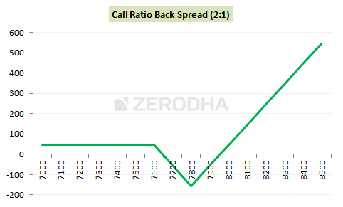
Notice how the payoff remains flat even when the market goes down, the maximum loss at 7800, and the way the payoff takes off beyond 7955.
4.4 – Welcome back the Greeks
I suppose you are familiar with these graphs by now. The following graphs show the profitability of the strategy considering the time to expiry and therefore these graphs help the trader select the right strikes.
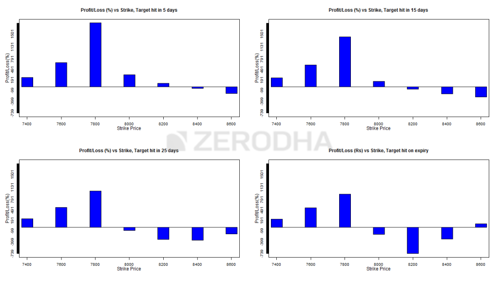
Before understanding the graphs above, note the following –
- Nifty spot is assumed to be at 8000
- Start of the series is defined as anytime during the first 15 days of the series
- End of the series is defined as anytime during the last 15 days of the series
- The Call Ratio Back Spread is optimized and the spread is created with 300 points difference
The thought here is that the market will move up by about 6.25% i.e from 8000 to 8500. So considering the move and the time to expiry, the graphs above suggest –
- Graph 1 (top left) and Graph 2 (top right) – You are at the start of the expiry series and you expect the move over the next 5 days (and 15 days in case of Graph 2), then a Call Ratio Spread with 7800 CE (ITM) and 8100 CE (OTM) is the most profitable wherein you would sell 7800 CE and buy 2 8100 CE. Do note – even though you would be right on the direction of movement, selecting other far OTM strikes call options tend to lose money
- Graph 3 (bottom left) and Graph 4 (bottom right) – You are at the start of the expiry series and you expect the move in 25 days (and expiry day in case of Graph 3), then a Call Ratio Spread with 7800 CE (ITM) and 8100 CE (OTM) is the most profitable wherein you would sell 7800 CE and buy 2 8100 CE.
You must be wondering that the selection of strikes is same irrespective of time to expiry. Well yes, in fact this is the point – Call ratio back spread works best when you sell slightly ITM option and buy slightly OTM option when there is ample time to expiry. In fact all other combinations lose money, especially the ones with far OTM options and especially when you expect the target to be achieved closer to the expiry.
Here are another bunch of charts; the only difference is that the move (i.e 6.25%) occurs during the 2nd half of the series –
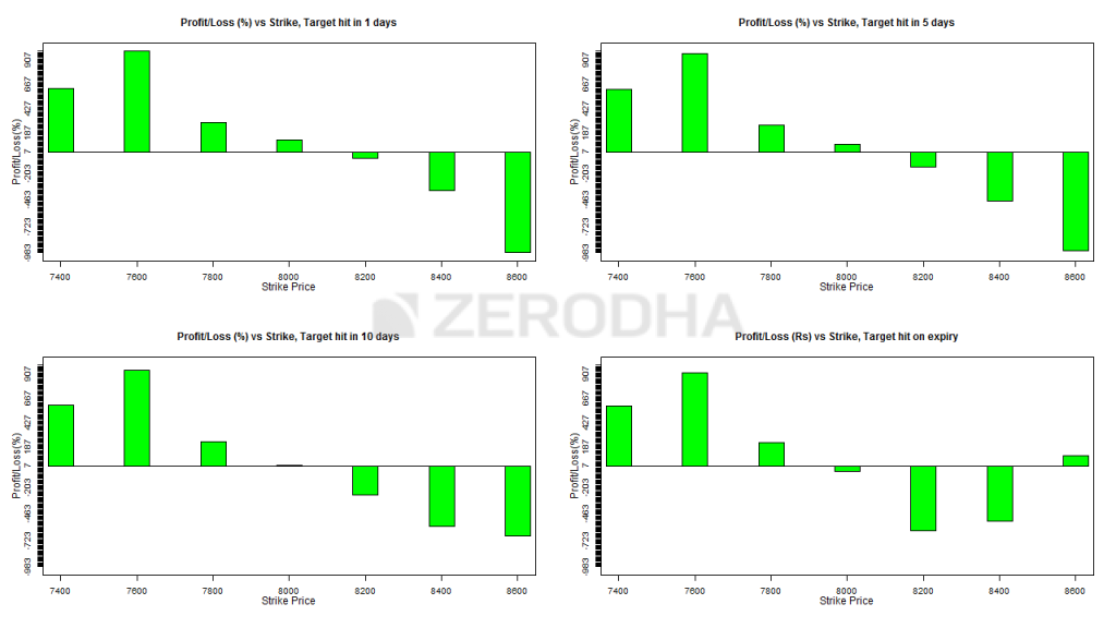
- Graph 1 (top left) & Graph 2 (top right) – If you expect the move during the 2nd half of the series, and you expect the move to happen within a day (or within 5 days, graph 2) then the best strikes to opt are deep ITM and slightly ITM i.e 7600 (lower strike short) and 7900 (higher strike long). Do note, this is not the classic combo of an ITM + OTM spread, instead this is an ITM and ITM spread! In fact all other combinations don’t work.
- Graph 3 (bottom right) & Graph 4 (bottom left) – If you expect the move during the 2nd half of the series, and you expect the move to happen within 10 days (or on expiry day, graph 4) then the best strikes to opt are deep ITM and slightly ITM i.e 7600 (lower strike short) and 7900 (higher strike long). This is similar to what graph 1 and graph 2 suggest.
Again, the point to note here is besides getting the direction right, the strike selection is the key to the profitability of this strategy. One needs to be diligent enough to map the time to expiry to the right strike to make sure that the strategy works in your favor.
What about the effect of volatility on this strategy? Well, volatility plays a key role here, have a look at the image below –
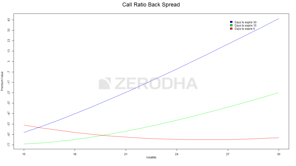
There are three colored lines depicting the change of “net premium” aka the strategy payoff versus change in volatility. These lines help us understand the effect of increase in volatility on the strategy keeping time to expiry in perspective.
- Blue Line – This line suggests that an increase in volatility when there is ample time to expiry (30 days) is beneficial for the Call ratio back spread. As we can see the strategy payoff increases from -67 to +43 when the volatility increase from 15% to 30%. Clearly this means that when there is ample time to expiry, besides being right on the direction of stock/index you also need to have a view on volatility. For this reason, even though I’m bullish on the stock, I would be a bit hesitant to deploy this strategy at the start of the series if the volatility is on the higher side (say more than double of the usual volatility reading)
- Green line – This line suggests that an increase in volatility when there are about 15 days time to expiry is beneficial, although not as much as in the previous case. As we can see the strategy payoff increases from -77 to -47 when the volatility increase from 15% to 30%.
- Red line – This is an interesting, counter intuitive outcome. When there are very few days to expiry, increase in volatility has a negative impact on the strategy! Think about it, increase in volatility when there are few days to expiry enhances the possibility of the option to expiry OTM, hence the premium decreases. So, if you are bullish on a stock / index with few days to expiry, and you also expect the volatility to increase during this period then thread cautiously.
Key takeaways from this chapter
- The Call Ratio Backspread is best executed when your outlook on the stock/index is bullish
- The strategy requires you to sell 1 ITM CE and buy 2 OTM CE, and this is to be executed in the same ratio i.e for every 1 sold option, 2 options have to be purchased
- The strategy is usually executed for a ‘net Credit’
- The strategy makes limited money if the stock price goes down, and unlimited profit if the stock price goes up. The loss is pre defined
- There are two break even points – lower breakeven and upper breakeven points
- Spread = Higher Strike – Lower Strike
- Net Credit = Premium Received for lower strike – 2*Premium of higher strike
- Max Loss = Spread – Net Credit
- Max Loss occurs at = Higher Strike
- The payoff when market goes down = Net Credit
- Lower Breakeven = Lower Strike + Net Credit
- Upper Breakeven = Higher Strike + Max Loss
- Irrespective of the time to expiry opt for slightly ITM + Slightly OTM combination of strikes
- Increase in volatility is good for this strategy when there is more time to expiry, but when there is less time to expiry, increase in volatility is not really good for this strategy.
Download Call Ratio Back Spread Excel Sheet
Thanks sir for this wonderful strategy . I am having two points here to ask.
1) Can we select the strike prices such that the spread and net credit are more or less same. So that the max. loss will be minimum. (Spread-net credit)? Is it practically possible to select premiums like that?
2) the pay off you have mentioned is adjusted against the time decay. It is more of concern when time to expiry is more.
Once again the topic is covered in a very simple way and easy to understand and grasp. .
Spread and Credit cannot be same. Net Credit is always lesser than the spread.
Time decay is not a good thing for this strategy, the only way it would works is when markets go higher.
What shall be practical minimum value for Max loss (spread- credit) so that it becomes worth taking position?
This depends on your risk appetite 🙂
1. Sir can you send payoff excel so that pay off calculation will be easy. [email protected] is id.
2. Does it gives profit intraday if upper and lower strike is crossed in intraday or time value also matters?
Thanks
Pawan
The excel can be downloaded at the end of the chapter, the link is provided.
You may experience an profit intraday, although holding this to expiry makes more sense.
Can we buy put instead of selling call?? I personally modified this strategy this way at zerodha and it worked well for me in volatile market. The beauty and versatality of option strategy is that you can always improvise…dont we??
Of course you can always improvise. Options are like white canvas, your imagination is the only limiting factor for what you can create on it.
Hi sir can I use this strategy for election result which is on may23 .
If the situation demands, then maybe you should 🙂
OK, I was asking that the charts shown here and in P/L calculation for month end etc, whether time decay is considered or not? If not then our P/L will be different.
Oh ok…time decay is considered since the chart depicts the payoff at expiry.
Hey karthik!!
Thank you very much to you and zerodha for varsity content!! Best on internet I must say!!
I can’t understand what graphs are conveying? i.e., target hits in 5, 10, 15, 25 and last day of expiry. Ofcourse they are showing the profits percentage but why they are above and below the x-axis. I’m totally confused. Please let me out of this confusion.
Thanks, Harsh.
Target hits in 5, 10, 15, 25 —- > these are the number of days in which the profit is supposed to hit.
Sir, How much margin for selling an itm option overnight.. Also is it possible to do this intra day.. I mean every day in a month.. We don’t keep risk of overnight news shocks and also margin requirements? Please enlighten
The margins will be similar to futures margin. Check our margin calculator here – https://zerodha.com/margin-calculator/SPAN/
There is no directional risk here for this strategy as either ways you make some money…the problem will be if the stock stays where it is. Also, this strategy is not really suitable for intraday.
Hey Karthik,
i just had a small doubt regarding the profitability graphs. There is a line that says “The following graphs show the profitability of the strategy:. So the graph for 7800 strike means- a call ratio back spread with a short 7800 strike Call and 2 long 8100 Calls? Just a little confused here
Absolutely!
Hi kartik
As I learn in option theory chapter, that today is Dec, then Dec. Is current month, Jan. Is mid month and Feb. Is far month. But in nifty we see good volumes in March, April,… Contracts. Is it possible to buy March, April,… Contracts when current month is Dec. ????
Can you please post a screen shot?
Why nifty has trade in April contract
These are quarterly contracts, here is an extract from NSE –
The Exchange shall introduce long term option contracts on NIFTY. The options cycle shall be as under.
The 3 serial month contracts would continue to exist.
The following 3 quarterly months of the cycle March / June / September / December would be available.
After these, 5 following semi-annual months of the cycle June / December would be available, so that at any point in time there would be options contracts with atleast 3 year tenure available
Thanks
That means if I have 6 month view on nifty I can buy quarterly contact and for 3 months we follow as above
Yes.